Exploring Argo Data Before You Write Code
OceanGraph helps you explore Argo float data before you start writing code.
When you begin oceanographic research, you are often told to “look at the data,” but it is not always clear what to look for or how to interpret what you see.
OceanGraph is a web-based visualization platform that lets you interactively browse Argo float profiles, trajectories, and θ-S diagrams, helping you build intuition and develop research questions without dealing with NetCDF files or complex scripts.
Open OceanGraph to explore real Argo profiles while reading this guide.
With OceanGraph, you can:
- Compare vertical profiles across locations and time
- Examine water mass characteristics using θ-S diagrams
- Trace float trajectories to understand spatial context
- Identify patterns and anomalies that may lead to research questions
OceanGraph is not a replacement for numerical analysis or scripting. It is designed to support early-stage exploration and interpretation, not to produce final results for publication.
Start Exploring
Features
For everyone
- Search Argo floats worldwide by region and time (up to a 30-day date range)
- Search only profiles that include at least one BGC parameter
- Search by WMO ID for direct access to specific floats
- Track individual float trajectories
- Visualize time-series vertical sections of Argo float data
Note: To prevent server overload, anonymous users are subject to request rate limits. If you experience rate limit restrictions, creating a free account and signing in will provide more generous rate limits for uninterrupted access.
For signed-in users
All free features, plus:
- Search Argo floats with an extended date range (up to 90 days)
- Visualize vertical profiles of temperature, salinity, oxygen, and supported BGC parameters
- View mixed layer depth from profile data
- View SOM (subsurface oxygen maximum) depth and its corresponding oxygen values
- Generate θ-S diagrams for search results with up to 500 profiles
- Download observation profile data for custom analysis
- Save screenshots of search results and visualizations
- Store up to 3 saved searches for repeated use (*)
- Bookmark up to 5 float profiles for later reference or comparison (*)
- Cluster Argo float profiles for pattern analysis with up to 500 profiles
- Browse Ocean Basins and Mode Waters views in Visual Lab
- Upload and compare up to 30 custom JSON profiles in Vertical Profiles (desktop browsers only)
(*) Titles can contain up to 64 characters, and notes up to 200 characters.
App Guide
This guide provides comprehensive information about using OceanGraph and understanding the data.
OceanGraph is a web application for searching and analyzing ocean observation data collected by the International Argo Program. You can search for temperature, salinity, dissolved oxygen, and other measurements from Argo floats based on geographic and temporal criteria, and explore the ocean state through various visualization and analysis features.
Open OceanGraph to follow this guide using the live application.
What’s in This Guide
Data Guide
Understand the data behind OceanGraph:
- Data Source: Data obtained from the International Argo Program’s Global Data Assembly Centre (GDAC)
- Data Filtering Policy: How quality-controlled, reliable profiles are selected (real-time and delayed-mode data, required variables, date and position quality checks)
- Limitations: Important considerations when interpreting data, such as missing values in vertical sections and sparse data due to quality control
Data is updated weekly, with approximately one week’s worth of new data typically added every weekend. Updates are announced on X (Twitter) at @OceanGraphJP.
Usage Guide
Learn how to use OceanGraph’s main features:
- Searching and Analyzing Argo Floats: Search for float profiles using geographic bounds, date ranges, and data quality conditions, then perform analyses including trajectories, time series, vertical sections, θ-S diagrams, clustering, mixed layer depth, subsurface oxygen maximum, and mode water map overlays
- Exploring Analysis Views: Browse precomputed Ocean Basins and Mode Waters views using Visual Lab
- Working with Custom Profiles: Upload Argo-format JSON files and compare vertical profiles using Analysis Lab
Start the Live App
Quick Start: Your First 10 Minutes
This page is a guided path for your first session with OceanGraph. It walks you from searching the map to exploring water masses and BGC-derived metrics, and links out to the detailed feature pages along the way.
Open OceanGraph and follow along.
What you can do without signing in
Search, WMO ID lookup, Trajectory View, and time-series View section work without an account. Signing in unlocks a longer search range and the analysis displays:
- Anonymous: search up to a 30-day range.
- Signed in: search up to a 90-day range, plus θ-S, Clustering, MLD, SOM, mode water map overlays, profile downloads, saved searches (up to 3), bookmarks (up to 5), and screenshots.
You can complete steps 1–3 below without signing in. Steps 4–5 require a signed-in account.
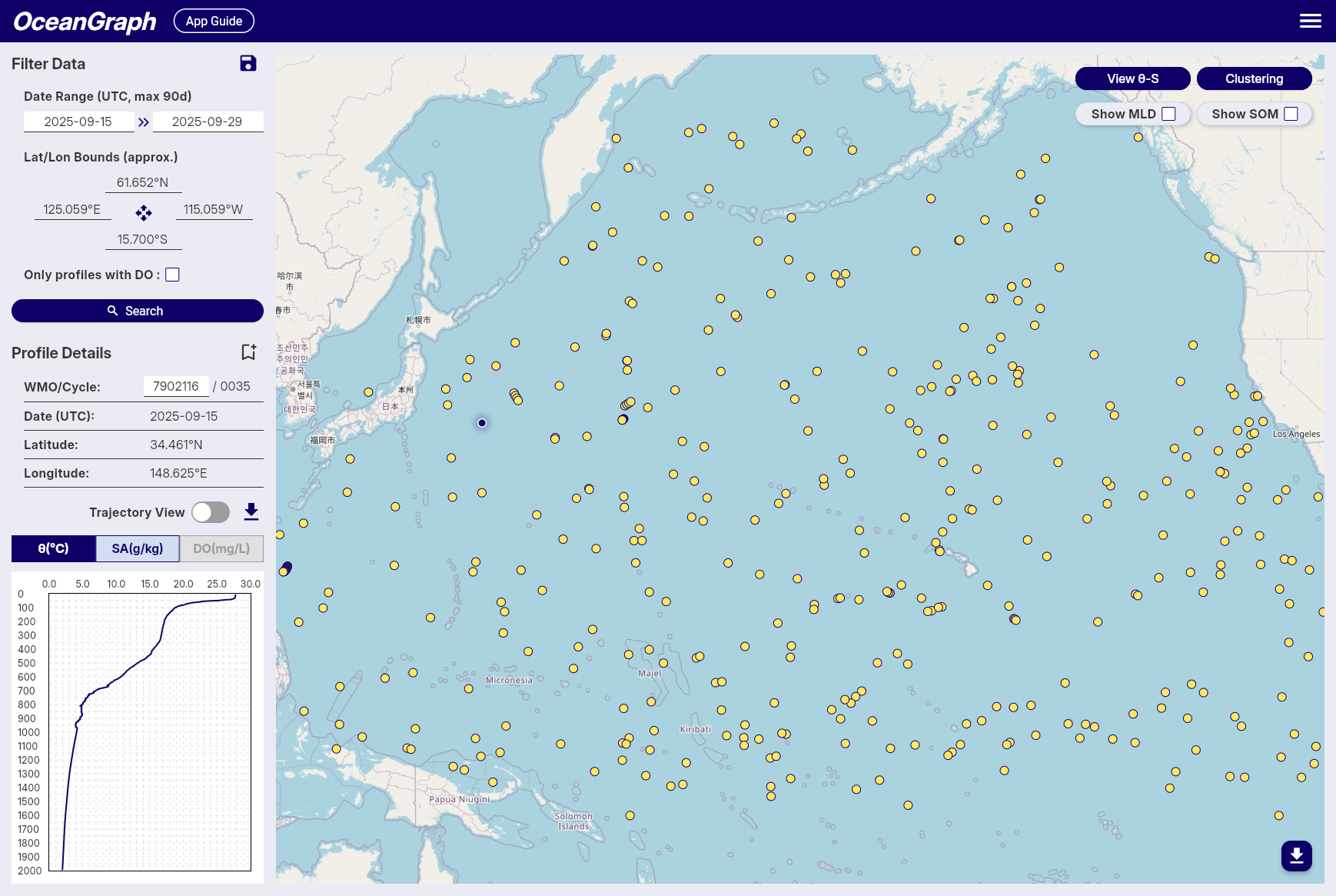
Step 1: Search the map
- Set a Date Range (anonymous: up to 30 days; signed in: up to 90 days).
- Set the Geographic Bounds by interacting with the map.
- Optionally check Only profiles with BGC to keep only profiles that include a biogeochemical parameter (dissolved oxygen, chlorophyll, nitrate, backscattering, pH, irradiance at 490 nm, or PAR).
- Run the search. Matching profiles appear as markers on the map.
If you already know a float, enter its WMO ID in the Profile Details panel and press Enter to load all of its profiles.
Too many results? Narrow the date range or geographic bounds. θ-S and Clustering accept at most 500 profiles, so a tighter search keeps those features available.
See Search and Bookmark for details.
Step 2: Select a marker
Click a marker to open its profile details (WMO ID, cycle number, date, latitude, longitude). Selecting a profile is the starting point for following a single float and for highlighting it in the analyses below.
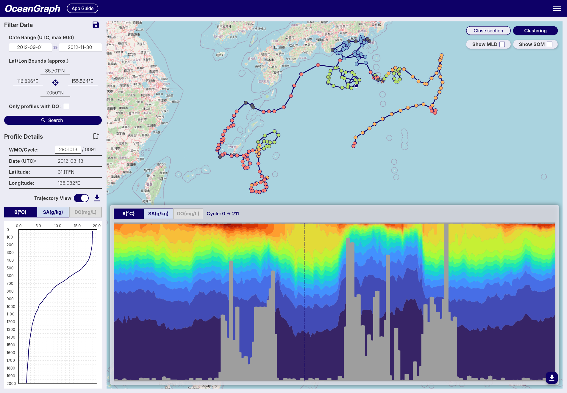
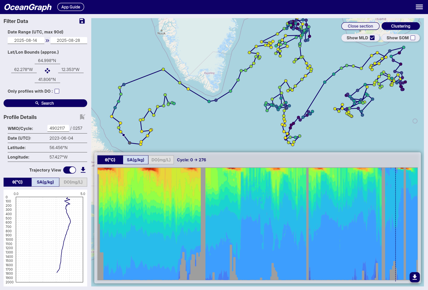
Step 3: Follow one float (Trajectory and Section)
- Turn on the Trajectory View switch to load profiles along the selected float’s trajectory.
- Click View section to see the time-series vertical section.
The dashed line on the section marks the currently selected profile. Gray or blank areas are places where data did not pass quality control (QC). BGC section charts appear only when the selected float carries that parameter.
See Trajectory and Time-Series Vertical Section.
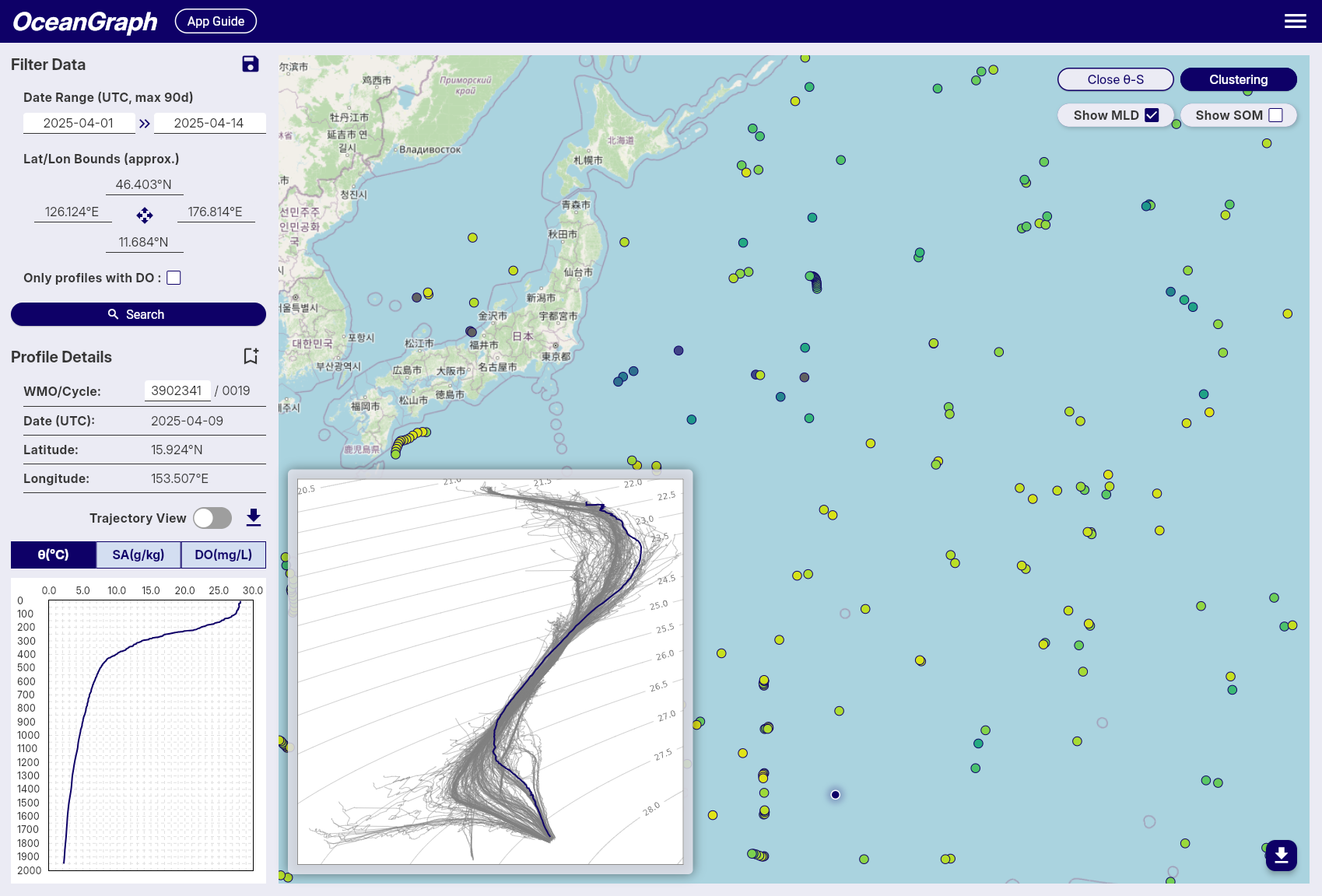
Step 4: Explore water masses (θ-S) — signed in
With a search active, click View θ-S in the top-right corner of the map to generate a θ-S diagram from the current results. Selecting a float on the map highlights its temperature-salinity line on the diagram. Click Close θ-S to hide it.
To group profiles by their vertical structure instead, click Clustering in the top-right corner and wait for the job to finish; markers are then colored by cluster. Both θ-S and Clustering accept a maximum of 500 profiles.
See θ-S Diagram and Clustering.
Step 5: Derived map overlays — signed in
Derived map overlays require a signed-in account and are shown via the map controls. Only one overlay can be active at a time.
- MLD — Open MLD / SOM and choose MLD. Mixed Layer Depth is computed from potential temperature, absolute salinity, and potential density. It does not require BGC data, so it works on core Argo profiles. Profiles with no valid MLD are shown in gray.
- SOM — Open MLD / SOM and choose SOM. Subsurface Oxygen Maximum requires dissolved oxygen, so it needs BGC profiles. Use Only profiles with BGC in your search first. Profiles without oxygen or a valid result are shown as no-data markers.
- Mode Water — Open Mode Water and choose a type such as NPSTMW or NASTMW. Profiles with the selected mode water are colored by detected layer thickness; profiles without that selected mode water are shown as no-data markers.
When Trajectory View and the matching section chart are open, MLD or SOM can also be overlaid on the section. Mode water coloring applies to map markers.
See Mixed Layer Depth (MLD), Subsurface Oxygen Maximum (SOM), and Mode Water Map Overlay.
If something doesn’t work
| Symptom | Likely cause and next step |
|---|---|
| No search results | The date range or area is too restrictive, or the BGC filter is on. Widen the range/area, or uncheck Only profiles with BGC. |
| θ-S or Clustering won’t run | Your search has more than 500 profiles. Narrow the date range or bounds. |
| A feature is missing from the screen | θ-S, Clustering, MLD, SOM, mode water overlays, and downloads require signing in. Sign in and try again. |
| BGC selected but a chart is missing | Not every BGC parameter has an in-app chart (e.g., irradiance at 490 nm is searchable and downloadable but not charted), and the float may not carry that parameter. |
| Vertical section is gray or blank | Those depths/times did not pass QC. See Limitations. |
| MLD, SOM, or mode water markers are gray / no-data | The profile lacks a valid derived result. For SOM, use BGC profiles with dissolved oxygen. For mode water, the selected type may not have been detected under the current criteria. |
| Vertical Profiles won’t open on mobile | Vertical Profiles is desktop-only. Open it on a desktop browser via Menu > Analysis Lab > Vertical Profiles. |
For more on why data can be sparse or missing, see Limitations.
Where to go next
- Compare your own Argo-format JSON files in Vertical Profiles (signed-in, desktop only).
- Browse precomputed views in Visual Lab.
- Read the Articles for background on Argo floats, T-S diagrams, BGC parameters, and more.
Data Guide
This section explains where OceanGraph data comes from, how profiles are filtered, and what limitations to keep in mind when interpreting results.
Open OceanGraph to inspect the live dataset while reading this guide.
Data is updated weekly, with approximately one week’s worth of new data typically added every weekend. Updates and notifications about data availability are posted on X (Twitter) at @OceanGraphJP.
Data Source
OceanGraph uses Argo float data and associated metadata provided by the International Argo Program and the national programs that contribute to it. These data are made freely available through the Argo Global Data Assembly Centre (Argo GDAC) and are a core component of the Global Ocean Observing System (GOOS).
For data access, OceanGraph retrieves Argo GDAC files via the public AWS S3 distribution (Open Data on AWS), which is synchronized with the GDAC holdings and updated on a daily basis. This S3-based access method is used to improve download reliability and performance, while preserving the original GDAC directory structure and dataset contents.
References:
- International Argo Program: https://argo.ucsd.edu
- OceanOPS Argo Information Centre: https://www.ocean-ops.org/board?t=argo
The former JCOMMOPS Argo Information Centre has been rebranded as OceanOPS.
Acknowledgement “These data were collected and made freely available by the International Argo Program and the national programs that contribute to it. (https://argo.ucsd.edu, https://www.ocean-ops.org). The Argo Program is part of the Global Ocean Observing System.”
DOI / Citation Argo (2000). Argo float data and metadata from Global Data Assembly Centre (Argo GDAC). SEANOE. https://doi.org/10.17882/42182
Data Filtering Policy
In OceanGraph, only carefully selected Argo float profiles are used according to the following conditions:
What this means for users
- OceanGraph does not display every profile that exists in the Argo GDAC. Profiles can be excluded by file type, quality control flags, missing required variables, depth coverage, pressure gaps, or conversion errors.
- When both real-time and delayed-mode data are available for the same cycle, delayed-mode data are preferred.
- BGC parameters are optional. A profile may appear in search results even if some BGC charts are unavailable.
- Missing areas in vertical section charts usually mean that the original data were unavailable, failed quality control, or were too sparse for interpolation.
- Adjusted data are used when complete adjusted pressure, temperature, and salinity are available; otherwise OceanGraph falls back to non-adjusted values.
1. Selection of profiles
1-1. File-level selection
- Only real-time (
R,BR) and delayed-mode (D,BD) profiles are used. - If both real-time and delayed-mode profiles exist for the same cycle, the delayed-mode profile (D or BD) is preferred.
- Drift profiles (those whose filename has a cycle number suffix ending in
D, e.g.R1234567_027D.nc) are excluded.
1-2. Best-profile selection within a file
Some NetCDF files contain multiple profiles (N_PROF > 1) — for example, when a float records both descending and ascending phases in the same cycle, or when a Bio-Argo file stores data from different BGC sensors as separate profiles.
Note: The file-level D/BD preference (section 1-1) and the within-file DATA_MODE-based selection (section 1-2) are independent mechanisms and may both apply to the same cycle.
TS profile selection
When a TS file contains more than one profile, the following algorithm selects the best candidate:
| Step | Type | Rule |
|---|---|---|
| Step 0 | Pre-filter | Candidates with invalid JULD_QC or POSITION_QC are removed. If all candidates fail, no filtering is applied at this step (they will be rejected in the QC stage below). |
| Step 1 | Hard rule | Profiles with DIRECTION == 'A' (ascending) are preferred. If no ascending profile exists, all remaining candidates are kept. |
| Step 2 | Hard rule | Profiles are filtered by DATA_MODE priority: D (delayed mode) > A (adjusted real-time) > R (real-time). |
| Step 3 | Tie-breaker | If multiple candidates remain, the profile with the highest quality score is selected. The score is based on the presence of _ADJUSTED data, the count of valid QC flags, and the valid pressure range. |
Steps 0–2 are hard rules that narrow down candidates according to Argo specification priorities. Step 3 (scoring) is used only when the hard rules cannot determine a single winner.
Why ascending profiles are preferred: Argo floats collect data primarily during the ascending phase. Sensors stabilize during ascent, and delayed-mode quality control (DMQC) targets ascending profiles. Ascending profiles are therefore preferred both physically and operationally.
BGC parameter selection
Bio-Argo files (BR/BD) have their own N_PROF dimension, independent of the corresponding TS file. Different BGC sensors may be stored as separate profiles within the same file due to sensor-specific processing — for example, DOXY in profile 0 and CHLA in profile 1. For this reason, each BGC parameter independently selects its own best profile rather than using a single shared index.
For each BGC parameter, the selection proceeds as follows:
- Profiles that contain valid data for the parameter (using
_ADJUSTEDif available, otherwise raw) are identified as candidates. - Candidates whose pressure levels match those of the selected TS profile (using raw
PRES) are retained. If no candidate matches, the parameter is treated as absent for that profile. - If multiple candidates remain, selection follows the same DIRECTION →
DATA_MODE→ tie-breaker scoring order as TS profile selection.
Note: The pressure matching in step 2 applies regardless of N_PROF. Even when a Bio-Argo file contains only one profile, if its pressure levels do not match those of the selected TS profile, the BGC parameter is treated as absent for that cycle.
2. Required variables
Only profiles that include all of the following variables are used:
PLATFORM_NUMBERCYCLE_NUMBERJULDJULD_QCLATITUDELONGITUDEPOSITION_QCPRESPRES_QCTEMPTEMP_QCPSALPSAL_QC
Note: The _ADJUSTED variables (PRES_ADJUSTED, TEMP_ADJUSTED, PSAL_ADJUSTED and their QC flags) are also included. When all three _ADJUSTED variables and their QC flags exist and each contains valid (non-NaN) data, the adjusted variables are used. Otherwise, the non-adjusted variables are used (see section 5 for details).
BGC parameters (optional): Bio-Argo profiles may additionally contain biogeochemical (BGC) parameters. These are not required for a profile to be included, but when present they are processed and made available. The supported BGC parameters are:
DOXY_ADJUSTED/DOXY_ADJUSTED_QC— Dissolved oxygen (μmol/kg)CHLA_ADJUSTED/CHLA_ADJUSTED_QC— Chlorophyll-a (mg/m³)NITRATE_ADJUSTED/NITRATE_ADJUSTED_QC— Nitrate (μmol/kg)BBP700_ADJUSTED/BBP700_ADJUSTED_QC— Particulate backscattering coefficient at 700 nm (m⁻¹)PH_IN_SITU_TOTAL_ADJUSTED/PH_IN_SITU_TOTAL_ADJUSTED_QC— pHDOWN_IRRADIANCE490_ADJUSTED/DOWN_IRRADIANCE490_ADJUSTED_QC— Downwelling irradiance at 490 nm (W/m²/nm)DOWNWELLING_PAR_ADJUSTED/DOWNWELLING_PAR_ADJUSTED_QC— Photosynthetically available radiation (μmol/m²/s)
A Bio-Argo file is considered valid if it contains at least one complete BGC parameter pair (either _ADJUSTED or non-adjusted variant).
Note: Of the two irradiance parameters, only PAR (DOWNWELLING_PAR) is currently available as an in-app visualization. Downwelling irradiance at 490 nm (DOWN_IRRADIANCE490) is processed and included in downloadable profile data, but is not displayed in the OceanGraph interface.
3. Date and position quality control
-
Only profiles with
JULD_QCvalues of 1, 2, or 8 are used. -
Only profiles with
POSITION_QCvalues of 1, 2, or 8 are used. -
Even if a profile passes the
POSITION_QCcheck, some data may still be unreliable. For example, as shown in the red circle below, caution is advised when interpreting such data.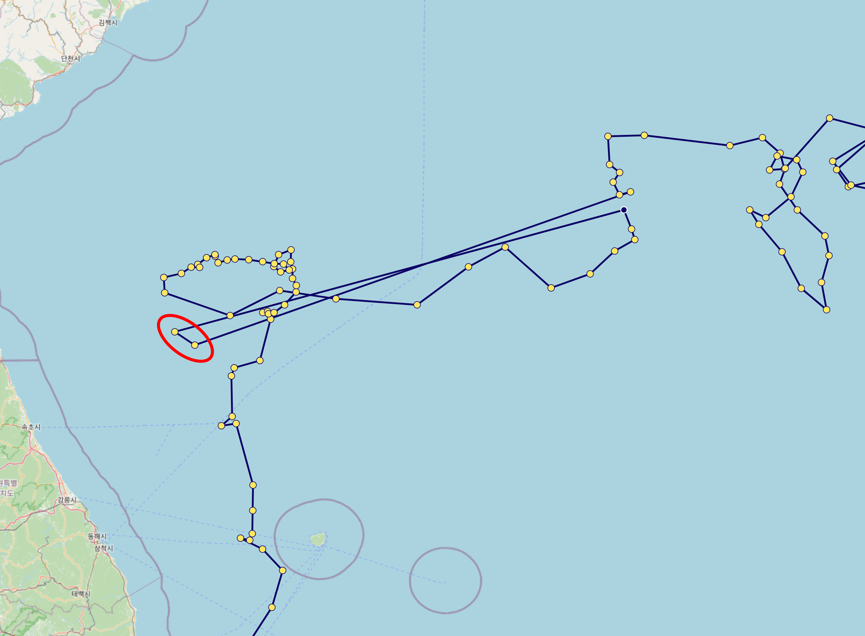
4. Longitude normalization
Some Argo profiles contain longitude values outside the standard range of -180° to 180°. To ensure consistent geographic positioning, longitude values are normalized to the [-180°, 180°] range during data processing.
- Longitude normalization is applied before decimal rounding
- The normalization preserves the actual geographic location (e.g., 190° is converted to -170°)
- Normalized values maintain the standard precision of 0.001° (approximately 111 meters)
5. Data selection: Adjusted vs. non-adjusted
The system uses the following logic to determine which data to use:
- Validate data availability: The system checks whether all three
_ADJUSTEDvariables (PRES_ADJUSTED,TEMP_ADJUSTED,PSAL_ADJUSTED) and their corresponding QC flags exist and each contains valid (non-NaN) data. - Use ADJUSTED data: If all conditions in step 1 are met, all ADJUSTED variables and their corresponding QC flags are used.
- Fallback to non-adjusted data: If any of the three ADJUSTED variables is missing or entirely NaN, the system uses the non-adjusted variables (
PRES,TEMP,PSAL) and their QC flags instead.
This mechanism ensures that real-time profiles or profiles that have not yet undergone delayed-mode quality control can still be utilized, maximizing data availability while maintaining quality standards.
Data pairs:
PRES_ADJUSTED→PRESTEMP_ADJUSTED→TEMPPSAL_ADJUSTED→PSALDOXY_ADJUSTED→DOXY(if applicable)CHLA_ADJUSTED→CHLA(if applicable)NITRATE_ADJUSTED→NITRATE(if applicable)BBP700_ADJUSTED→BBP700(if applicable)PH_IN_SITU_TOTAL_ADJUSTED→PH_IN_SITU_TOTAL(if applicable)DOWN_IRRADIANCE490_ADJUSTED→DOWN_IRRADIANCE490(if applicable)DOWNWELLING_PAR_ADJUSTED→DOWNWELLING_PAR(if applicable)
The corresponding QC flags also follow the same fallback logic (e.g., PRES_ADJUSTED_QC → PRES_QC).
Note: For BGC parameters, each parameter independently determines whether to use the ADJUSTED or non-adjusted variant. Within the same profile, some BGC parameters may use ADJUSTED data while others fall back to non-adjusted data, depending on availability.
6. Depth range restriction
Only data from depths shallower than 2000 dbar are retained. Additionally, layers with negative pressure values are removed along with their corresponding data (temperature, salinity, dissolved oxygen, etc.).
7. Profile quality filtering
Only profiles where at least 80% of pressure, temperature, and salinity QC flags are 1, 2, or 8 are kept.
8. Layer-by-Layer filtering
Core variables (pressure, temperature, salinity):
Only layers where all QC flags for pressure, temperature, and salinity are 1, 2, or 8 are kept. These valid layers define the index set used for all subsequent variable selection, including BGC parameters.
BGC parameters (dissolved oxygen and other biogeochemical variables):
All BGC parameters are filtered in two stages:
Stage 1 — Profile-level QC threshold:
Before selecting layers, each BGC parameter’s QC flags are checked across the entire profile. If a parameter fails this check, its data is discarded for that profile (set to empty); the profile itself is not rejected.
- Dissolved oxygen, chlorophyll, nitrate, backscattering, and pH (
DOXY,CHLA,NITRATE,BBP700,PH_IN_SITU_TOTAL): data is discarded if fewer than 80% of QC flags pass (values 1, 2, or 8). - Irradiance parameters (
DOWN_IRRADIANCE490,DOWNWELLING_PAR): because these sensors only measure in the surface layer (roughly 0–200 dbar), most values in a deep profile are inherently NaN or invalid. Applying the 80% threshold would discard nearly all irradiance profiles. Instead, data is retained if at least one QC flag passes; if none pass, the data is discarded.
Stage 2 — Layer selection using core variable indices:
After the profile-level check, each BGC parameter is subsetted to the valid layers determined by the pressure/temperature/salinity QC above. The BGC parameters’ own QC flags are not used for individual layer selection — only the core variable indices determine which layers are kept.
The table below illustrates this logic (shown with dissolved oxygen, but the same applies to all BGC parameters):
| pres_qc | temp_qc | psal_qc | bgc_qc | Judgment |
|---|---|---|---|---|
| 1, 2, or 8 | 1, 2, or 8 | 1, 2, or 8 | any | PASS |
| 0 | 1, 2, or 8 | 1, 2, or 8 | any | FAIL |
| 1, 2, or 8 | 0 | 1, 2, or 8 | any | FAIL |
| 1, 2, or 8 | 1, 2, or 8 | 0 | any | FAIL |
BGC QC flags are not used for individual layer selection.
Note: BGC sensor data, dissolved oxygen in particular, may contain measurement uncertainties. Users should interpret BGC data carefully.
9. NaN value detection
After the layer-by-layer filtering, the system checks for any remaining NaN (Not a Number) values in the core variables:
- Pressure
- Temperature
- Salinity
If any NaN values are detected in these critical variables, the entire profile is rejected and removed from the dataset. This ensures data integrity and prevents computational errors in downstream analysis.
10. Physical bounds masking for BGC parameters
Before interpolation, each BGC parameter value is checked against a configured physical range (valid_min / valid_max). Any value that falls outside this range is replaced with None (treated as missing) — it is not clamped to the boundary value. These masked values are then filled in by the subsequent interpolation step (section 11), so the output JSON contains an interpolated estimate rather than the physically implausible raw value.
This step is independent of QC flag filtering. QC flags indicate measurement reliability as assessed by the data provider, but a value can carry a passing QC flag while still being physically impossible (e.g., DOXY = −634 μmol/kg). Physical bounds masking acts as an additional safeguard against such sensor anomalies that QC flags alone do not catch.
Current bounds configuration:
| Parameter | valid_min | valid_max | Notes |
|---|---|---|---|
DOXY | 0.0 μmol/kg | 600.0 μmol/kg | Physically impossible negative or extreme values have been observed |
CHLA, NITRATE, BBP700, PH_IN_SITU_TOTAL, DOWN_IRRADIANCE490, DOWNWELLING_PAR | — | — | No bounds currently applied |
Only DOXY has specific bounds configured at this time. Other parameters retain their current values unless bounds are explicitly set in the future.
Important note for irradiance parameters: DOWN_IRRADIANCE490 and DOWNWELLING_PAR use edge-preserving interpolation (no extrapolation at profile boundaries — see section 11). If a masked value falls at the leading or trailing edge of the profile, it will remain as null in the output JSON rather than being filled by interpolation.
11. Interpolation of missing values for BGC parameters
BGC parameters often contain missing (NaN) values. The interpolation procedure varies by parameter type:
Dissolved oxygen, chlorophyll, nitrate, backscattering, and pH (DOXY, CHLA, NITRATE, BBP700, PH_IN_SITU_TOTAL):
- Linear interpolation is used for internal (non-endpoint) missing values.
- Remaining missing values at the beginning or end of the profile are filled using backward-fill and forward-fill, respectively.
Irradiance parameters (DOWN_IRRADIANCE490, DOWNWELLING_PAR):
- Linear interpolation is used for internal missing values only.
- Missing values at the edges of the profile are not filled. Leading and trailing NaN values are physically meaningful — deep-water values are NaN because light does not penetrate to depth, and surface values may be NaN due to nighttime observations. These are preserved as
nullin the output JSON. - If all values remain
nullafter interpolation, the parameter is treated as absent for that profile.
12. Duplicate pressure value removal
To ensure data integrity and maintain strictly increasing pressure sequences, duplicate pressure values are removed using a deterministic sorting approach:
- Pressure grouping: Data points are grouped by rounded pressure values (to 0.01 dbar precision).
- Deterministic selection: When multiple data points exist at the same pressure level, they are sorted by:
- Original pressure value
- Temperature value
- Salinity value
- First entry retention: The first entry from the sorted group is kept, while duplicates are discarded.
This process ensures that each profile has a unique, monotonically increasing pressure sequence, which is essential for accurate oceanographic analysis and prevents computational issues in downstream processing.
13. Pressure gap filtering
Profiles with excessively large gaps in pressure measurements are rejected and removed from the dataset to ensure data continuity. The filtering uses depth-dependent gap thresholds that become more permissive with increasing depth:
- 0-100 dbar: Maximum gap of 33.33 dbar
- 100-200 dbar: Maximum gap of 66.67 dbar
- 200-300 dbar: Maximum gap of 100 dbar
- 300-1000 dbar: Maximum gap increases proportionally (depth/3)
- >1000 dbar: Maximum gap of 500 dbar
This ensures that profiles maintain adequate vertical resolution throughout the water column, with stricter requirements in shallower waters where oceanographic gradients are typically steeper.
14. Oceanographic parameter conversion
To ensure consistency with oceanographic standards, the following parameter conversions are applied:
- Temperature to potential temperature (θ): In-situ temperature is converted to potential temperature using the TEOS-10 Gibbs Seawater (GSW) oceanographic toolbox.
- Practical salinity to absolute salinity (SA): Practical salinity is converted to absolute salinity using the GSW toolbox, taking into account the geographic location (latitude/longitude) and pressure.
These conversions provide more accurate representations of water mass properties by removing the effects of pressure and enabling precise oceanographic calculations. Profiles that encounter computational errors during these conversions are rejected to maintain data quality.
15. Decimal precision
To reduce data size, the values are rounded to the nearest values shown below:
| Variable | Precision |
|---|---|
| Pressure | 0.01 |
| Temperature | 0.001 |
| Salinity | 0.001 |
| Dissolved oxygen concentration | 0.001 |
| Chlorophyll-a | 0.001 |
| Nitrate | 0.01 |
| Backscattering (BBP700) | 0.000001 |
| pH | 0.001 |
| Irradiance (490 nm) | 0.001 |
| PAR | 0.1 |
Limitations
Missing Values in Vertical Section Charts
-
Masked Areas Without Original Data
When generating time-series vertical section charts of Argo float data, linear 1D interpolation is used in two steps: first each profile is interpolated onto a common pressure grid, then values are interpolated along the cycle/time direction. Some areas may remain unfilled where original profile data are missing. To address this, masks are applied after interpolation to exclude regions without valid observations, setting those values to NaN.
In the example image below, these masked areas appear as uncolored gaps in the vertical section.
-
Sparse Data Due to Quality Control
After applying quality control, some profiles may be excluded, resulting in a sparser time series. Even if valid profiles are present at certain time steps, the interpolation process may not be able to generate a continuous vertical section. This leads to sections where observation points exist (trajectory figure) but the interpolated chart shows gray or missing areas (vertical section figure), indicating insufficient data density for interpolation.
This can be seen in the same image where gray regions appear in the section chart, even though observation points are visible in the trajectory chart above.
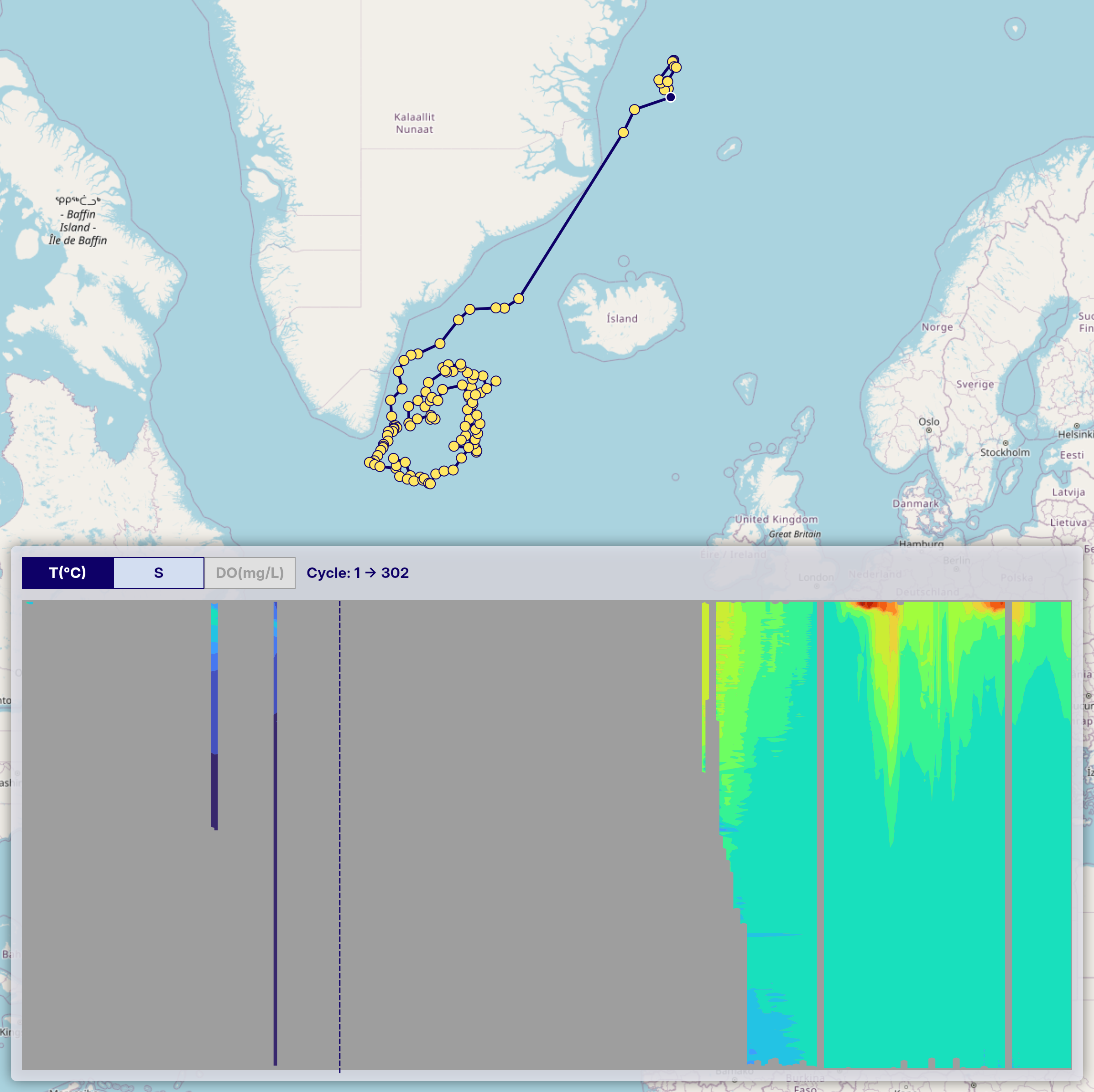
Please keep this in mind when interpreting the charts.
-
BGC Parameter Charts May Have More Missing Areas
Vertical section charts in the OceanGraph interface are also available for BGC parameters (chlorophyll, nitrate, backscattering, pH, and PAR). Because only a subset of Argo floats carry BGC sensors, BGC data is available for fewer floats overall compared to temperature or salinity. For a section chart of a specific float that does carry a BGC sensor, the number of cycles with BGC data is generally the same as for physical parameters — however, quality control may still cause some individual cycles to be discarded, which can result in gaps.
Additionally, PAR profiles contain data only in the surface layer (roughly 0–200 dbar). Deeper portions of PAR section charts will always appear as missing areas, which is physically expected behavior.
Note also that of the two irradiance parameters (
DOWN_IRRADIANCE490andDOWNWELLING_PAR), only PAR is displayed as an in-app chart. Downwelling irradiance at 490 nm can make a profile match the “Only profiles with BGC” search filter and is included in downloadable profile data, but it does not have a corresponding in-app visualization.
Derived Metrics and Mode Water Detection
Derived metrics such as MLD, SOM, and mode water detections are calculated automatically from profiles that pass OceanGraph’s data processing checks. A no-data marker can mean that the source profile was insufficient for the calculation, or that the target feature was not detected under the current criteria.
Mode water detection uses fixed geographic, density, potential vorticity, and minimum-thickness criteria. The default geographic scope is configured to cover broader areas that can include advected mode water signals, but it is still an automatic bounding-box screen and may not cover every scientifically relevant signal. Treat the map overlay and Visual Lab summaries as exploration aids, and inspect the original profile structure when a research-grade classification is required.
Usage Guide
This section guides you through OceanGraph’s core functionality, from searching for Argo float data to visualizing and analyzing oceanographic observations.
Open OceanGraph to follow these workflows with real Argo data.
OceanGraph provides three main workflows:
Basic Features
Start by searching for Argo float profiles using geographic bounds, date ranges, and data quality filters. Once you’ve found profiles of interest, you can:
- View float trajectories and bookmark profiles for later analysis
- Generate time-series vertical sections showing how temperature, salinity, and other parameters evolve
- Create θ-S diagrams to identify water masses
- Apply clustering analysis to group similar profiles
- View derived map overlays for mixed layer depth, subsurface oxygen maximum, and profile-level mode water detections
Some analysis and export features in this section require signing in, including θ-S diagrams, clustering, MLD, SOM, mode water map overlays, profile downloads, saved searches, bookmarks, and screenshots.
Visual Lab
Use Visual Lab to browse precomputed views of large-scale ocean patterns. The current Visual Lab pages are Ocean Basins and Mode Waters, both available to signed-in users from the app menu.
Analysis Lab
Analysis Lab provides tools for working with your own Argo-format profile data. The current Vertical Profiles tool lets signed-in desktop users upload JSON files, compare profile plots, add a note for exported files, and download charts.
Open OceanGraph
Basic Features
This section provides detailed guides for the core features of OceanGraph. These features enable you to search, visualize, and analyze Argo float data effectively.
Open OceanGraph to try these features in the live app.
Search, WMO ID lookup, trajectory display, and time-series vertical sections are available without signing in. θ-S diagrams, clustering, MLD, SOM, mode water map overlays, profile downloads, saved searches, bookmarks, and screenshots require a signed-in account.
Search and Bookmark allows you to find Argo float profiles using geographic, temporal, and data quality criteria, and bookmark profiles for future reference.
Trajectory and Time-Series Vertical Section visualizes how oceanographic parameters change with depth and time along a float’s trajectory, providing a comprehensive view of the water column structure throughout the float’s journey.
θ-S Diagram helps you explore potential temperature-absolute salinity relationships of Argo float profiles in your search area, enabling identification of water masses and their characteristics.
Clustering uses machine learning to group Argo profiles based on their vertical structure. This experimental feature helps identify similar oceanographic conditions across multiple profiles.
Mixed Layer Depth (MLD) calculates the mixed layer depth from Argo float profiles using multiple oceanographic parameters (potential temperature, absolute salinity, and potential density) with the Gibbs SeaWater Oceanographic Toolbox.
Subsurface Oxygen Maximum (SOM) identifies and analyzes the subsurface oxygen maximum layer, which characterizes the vertical structure of dissolved oxygen, particularly in subtropical and tropical regions.
Mode Water Map Overlay colors search-result map markers by profile-level mode water detection, helping you compare detected layer thickness for selected water masses such as NPSTMW, NASTMW, or IOSTMW.
Search and Bookmark
OceanGraph provides search capabilities to find Argo float profiles based on geographic, temporal, and data quality criteria.
Search Methods
Filter Data Panel
-
Date Range
- Available: October 1999 to present
- Click date fields to select start and end dates
- All times in UTC
- Anonymous users can search up to a 30-day range; signed-in users can search up to a 90-day range
-
Geographic Bounds
- Set by interacting with the map
- Coordinates displayed with N/S/E/W format
-
Data Availability
- “Only profiles with BGC” checkbox for profiles that include at least one supported BGC parameter: dissolved oxygen, chlorophyll, nitrate, backscattering, pH, downwelling irradiance at 490 nm, or PAR
- Not every BGC parameter has an in-app chart. Downwelling irradiance at 490 nm can be included in search and downloaded profile data, but it is not currently displayed as a chart.
-
Save Searches
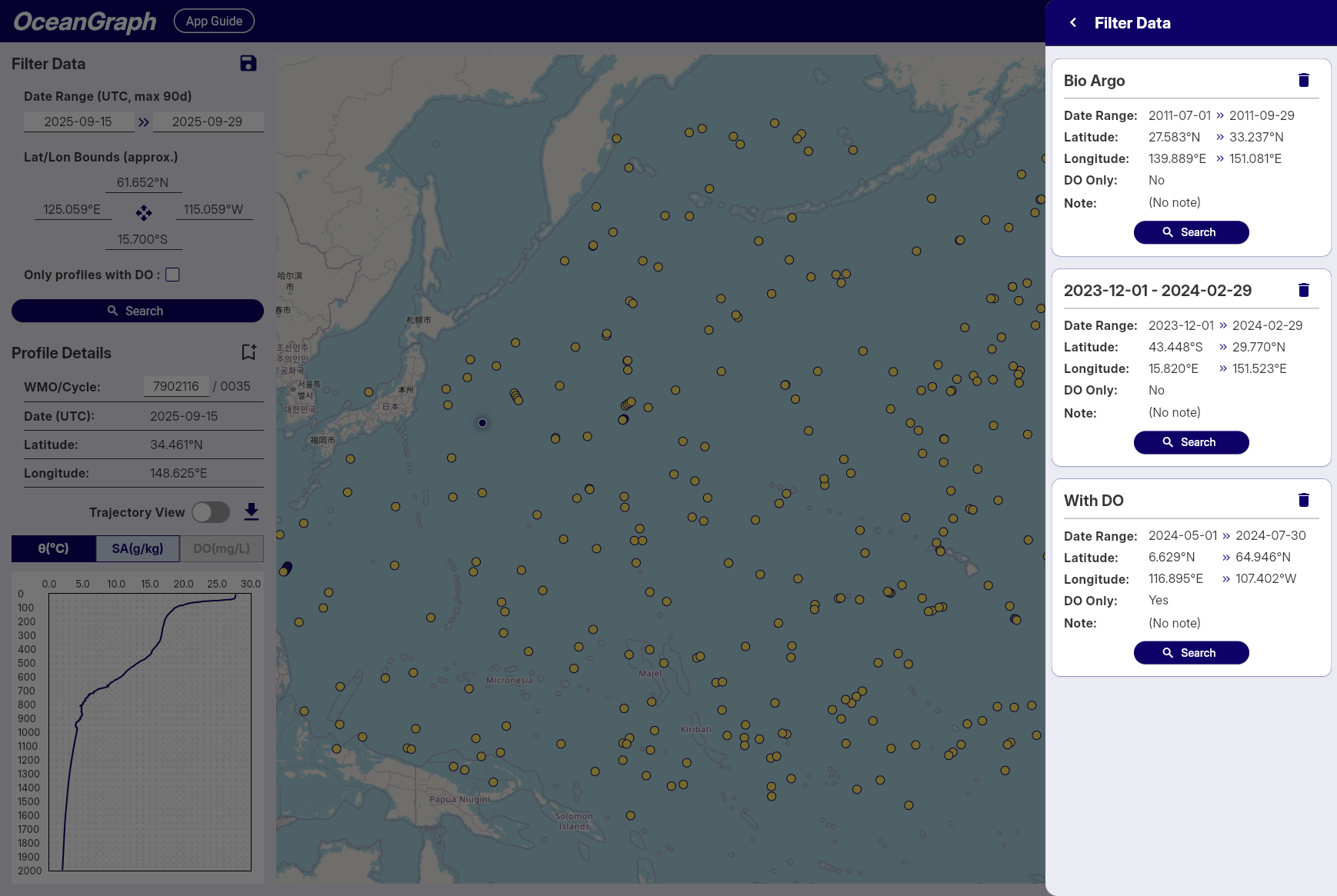
Note: Available to signed-in users only
- Click the save icon to save the current search parameters
- Automatic naming by date range
- Access saved searches across sessions
- Up to 3 saved searches can be stored
- The title (up to 64 characters) and an optional note (up to 200 characters) can be edited on each saved search
Profile Details Panel
-
WMO ID Search
- Enter WMO ID and press Enter
- Returns all profiles for that specific float
-
Profile Information
- WMO ID, Cycle Number, Date (UTC), Latitude, Longitude
-
Bookmark Profiles
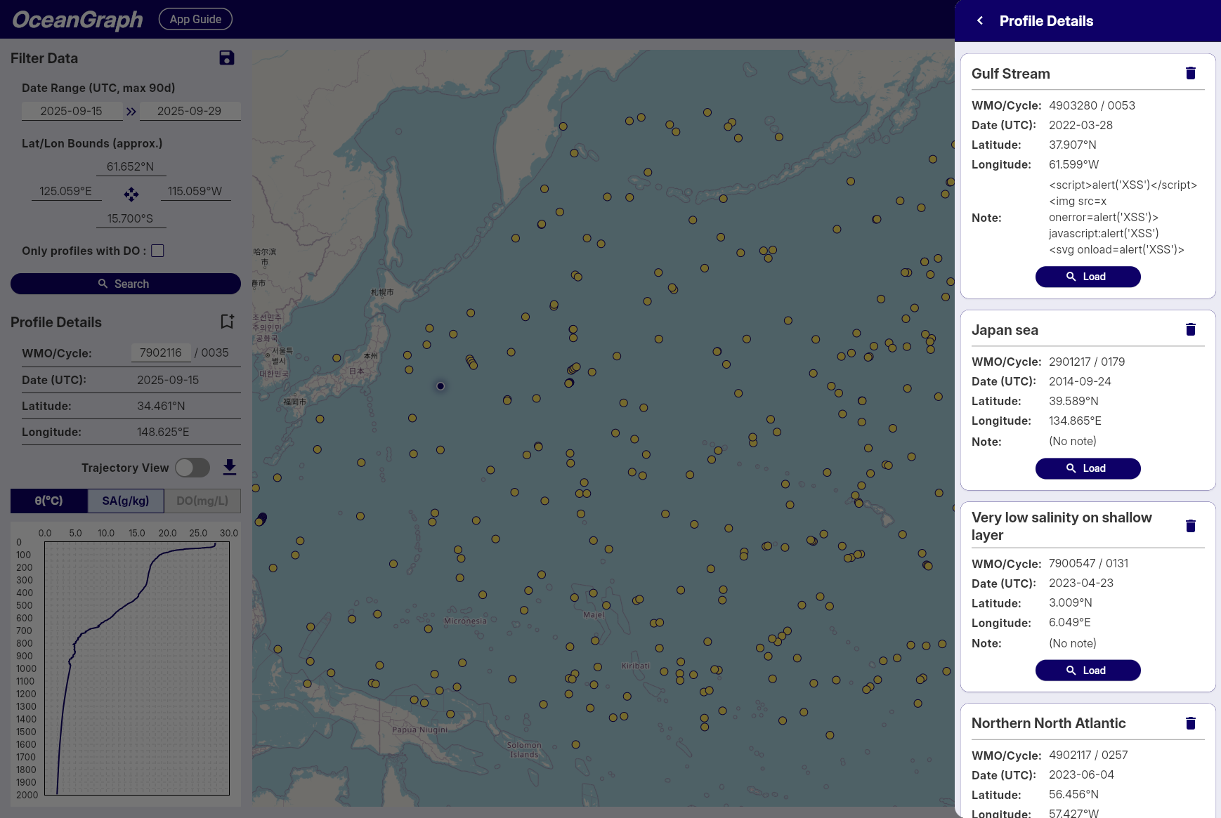
Note: Available to signed-in users only
- Click the bookmark icon to save profiles
- A status indicator shows which profiles are already bookmarked, preventing duplicates
- Access bookmarks across sessions
- Up to 5 profiles can be bookmarked
- The title (up to 64 characters) and an optional note (up to 200 characters) can be edited on each bookmarked profile
Search Results
- Result count notification
- Profiles displayed as map markers
- Click markers to view profile details
Tips
- Start with broad searches, then narrow down
- Use the BGC filter when you need profiles with biogeochemical measurements
- Save frequently used search patterns
- Bookmark important profiles for future reference
- Rate Limits: Signed-in users enjoy higher rate limits. If you experience access restrictions, consider creating a free account for uninterrupted access.
Trajectory and Time-Series Vertical Section
This feature allows you to visualize Argo float data as a time-series vertical section, showing how oceanographic parameters change with depth and time along the float’s trajectory. The vertical section provides a comprehensive view of the water column structure throughout the float’s journey.
Accessing Time-Series Vertical Sections
To access time-series vertical sections of Argo float data, follow these steps:
- Select a Float: Start by selecting an Argo float from the search results or the map view.
- Turn on Trajectory View: Turn on the “Trajectory View” switch to load profiles from the selected float’s trajectory.
- Show vertical section: Click the “View section” button to view the time-series data for the selected float.
Tips
- The vertical section is linked with the vertical profiles in Profile Details, and the position of the selected profile is shown with a dashed line.
- Missing data areas indicate locations where data did not pass quality control (QC).
- BGC section charts are shown only when the selected float has that parameter available.
- Signed-in users can overlay MLD or SOM on the section chart when the corresponding mode is active.
θ-S Diagram
The θ-S diagram feature allows you to visualize potential temperature-absolute salinity relationships of Argo float profiles in the current search area.
Accessing θ-S Diagram
The θ-S diagram is available to signed-in users only.
- Sign in and perform a search
- Click the View θ-S button in the top-right corner of the map
- The system will generate a θ-S diagram based on the current search results
- The diagram appears as an overlay on the map
- Click Close θ-S to hide the diagram
Profile Limit
- Maximum 500 profiles can be used to generate a θ-S diagram
- If your search contains more than 500 profiles, an error message will appear
- Narrow your search criteria to reduce the number of profiles
θ-S Diagram Display
Background Chart
- Shows potential temperature (vertical axis) vs absolute salinity (horizontal axis) relationships
- Displays density contour lines as background context
Selected Profile Line
- When you select a float on the map, its temperature-salinity profile is highlighted
- Appears as a colored line overlaying the background chart
- Updates automatically when you select different floats
Tips
- Use it to identify different water masses and their characteristics
- The diagram helps understand the oceanographic context of your selected profiles
Background
A θ-S diagram (Temperature-Salinity diagram) is a fundamental tool in oceanography for:
- Identifying water masses and their properties
- Understanding mixing processes between different water types
- Analyzing the vertical structure of the water column
- Detecting seasonal and regional variations in ocean properties
Clustering
OceanGraph provides an experimental feature that clusters Argo profiles based on their vertical structure using machine learning. This functionality is experimental and comes with the following limitations and processing steps:
Note: Gray markers indicate profiles that were excluded from clustering.
Accessing Clustering
Clustering is available to signed-in users only.
- Sign in and perform a search
- Narrow the search results to 500 profiles or fewer
- Click the Clustering button in the top-right corner of the map
- Wait for the job to complete; the map markers are colored by cluster
If a clustering job takes too long, use the cancel control shown during processing. If polling fails, retry from the status message.
Interpreting Results
- Colored markers indicate profiles assigned to clusters.
- Gray markers indicate profiles excluded from clustering because they did not satisfy the required variables or depth coverage.
- The cluster labels are exploratory groups, not confirmed water-mass names.
Processing Details
-
Profile Limit
- To reduce server load and memory usage, clustering accepts a maximum of 500 valid profiles per job.
-
Depth Range & Interpolation
- The depth range used for clustering is dynamically determined based on the input profiles:
- Minimum depth: Fixed at 200 dbar to suppress the effects of seasonal thermocline and surface forcing.
- Maximum depth: Automatically set to the 25th percentile of maximum depths across all valid profiles, then rounded down to the nearest 100 dbar increment.
- If the calculated maximum depth is greater than 200 dbar and less than 1000 dbar, that value is used. Otherwise, the maximum depth falls back to 1000 dbar.
- Profiles that do not cover the selected depth range are excluded from clustering.
- Profiles are linearly interpolated every 100 dbar within this determined range to align them on a common vertical grid.
- This adaptive approach ensures optimal clustering performance regardless of the depth characteristics of the selected profiles.
- The depth range used for clustering is dynamically determined based on the input profiles:
-
Required Variables
- Only profiles containing valid temperature and salinity data are considered.
- Profiles missing these variables or lacking coverage in the specified depth range are excluded.
-
Clustering Feature Vector
- Clustering is based on a feature vector composed of interpolated temperature and salinity values, combined with location data.
- Temperature and salinity vectors are standardized using z-score normalization at each depth level to ensure that variations at all depths contribute equally to the clustering process.
- Latitude is included as an additional feature, normalized by linear scaling from -90 to 90 degrees into a range of -1 to 1.
- Longitude is transformed into two features using its sine and cosine values (i.e., sin(λ), cos(λ)), allowing for circular continuity around the ±180° meridian without further normalization.
-
Automatic K Determination
- The number of clusters (K) is selected automatically using a simplified elbow method (with a maximum of 6 clusters).
Mixed Layer Depth (MLD)
OceanGraph calculates the mixed layer depth (MLD) from individual Argo float profiles using multiple threshold criteria based on potential temperature (θ), absolute salinity, and potential density (σθ). Potential temperature, absolute salinity, and density are calculated with the Gibbs SeaWater (GSW) Oceanographic Toolbox for accurate thermodynamic calculations.
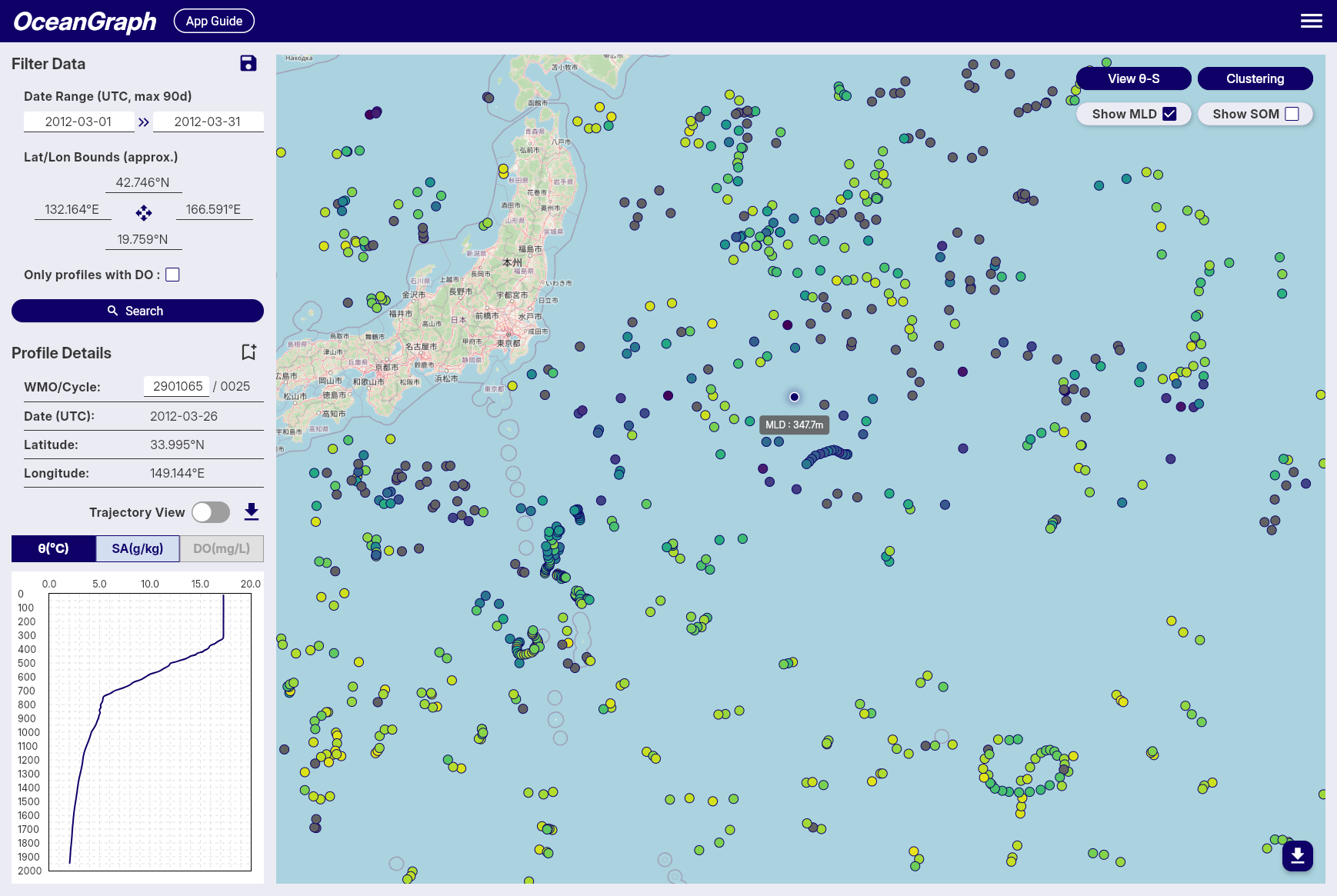
Accessing MLD
MLD display is available to signed-in users only.
- Sign in and perform a search
- Open MLD / SOM in the map controls and choose MLD
- Use the marker colors and tooltips to compare mixed layer depth across profiles
MLD, SOM, and mode water map overlays are mutually exclusive. Selecting MLD turns off SOM and mode water coloring. Profiles with missing or undefined MLD values are rendered in gray.
When Trajectory View and the section chart are open, selecting MLD also overlays an MLD line on the vertical section.
Calculation Details
-
Multi-Parameter Calculation
- MLD is determined using three different oceanographic parameters: potential temperature (θ), absolute salinity, and potential density (σθ).
- Potential temperature and density are calculated using the GSW toolbox based on practical salinity, in-situ temperature, pressure, and latitude.
- This ensures high accuracy and consistency in the estimation of stratification and mixed layer properties across different oceanographic conditions.
-
MLD Definition and Threshold
- The MLD is calculated using three different threshold criteria and defined as the shallowest depth among the three methods:
- Temperature threshold (Δθ): Depth where potential temperature (θ) differs by more than 0.5°C from its value at 10 dbar
- Salinity threshold (ΔSA): Depth where absolute salinity differs by more than 0.05 g/kg from its value at 10 dbar
- Density threshold (Δσθ): Depth where potential density (σθ) differs by more than 0.125 kg/m³ from its value at 10 dbar
- This multi-parameter approach provides a more robust estimation of the mixed layer depth by considering both thermal and haline stratification.
- If no depth is found using any of the three criteria, the MLD is considered undefined for that observation.
- The MLD is calculated using three different threshold criteria and defined as the shallowest depth among the three methods:
-
Data Quality Requirements
- Reference Depth Coverage: The shallowest observation must be no more than 20 dbar deeper than the reference depth (10 dbar). If this condition is not met, or if the reference depth is deeper than the deepest observation, MLD calculation is skipped for that profile. When the shallowest observation is within 20 dbar of the reference depth, the shallowest observed value is used as the surface representative value for the MLD calculation.
- Shallow Data Availability: A minimum of 2 data points at or above 50 dbar is required for reliable MLD calculation. Profiles with insufficient shallow measurements are excluded from MLD computation to ensure accuracy.
-
Conversion to Depth
- The estimated MLD (in decibars) is converted into physical depth (in meters) using a latitude-dependent algorithm from the UNESCO 1983 standard.
- This conversion allows MLD values to be spatially visualized or regionally compared using consistent units.
-
Color Representation
- For visualizations such as maps, MLD values are mapped to colors using the cmocean
deepcolormap. - Profiles with missing or undefined MLD values are rendered in gray.
- For visualizations such as maps, MLD values are mapped to colors using the cmocean
This approach provides an accurate and robust estimation of mixed layer depth across a wide range of Argo float profiles by utilizing multiple oceanographic parameters. The multi-threshold method ensures that the MLD estimation captures both thermal and haline stratification effects, making it particularly well-suited for visual analysis and regional comparisons in diverse oceanographic environments.
Subsurface Oxygen Maximum (SOM)
OceanGraph calculates the subsurface oxygen maximum (SOM) for individual Argo float profiles using dissolved oxygen and pressure (or depth) data. This metric is widely used in oceanography to characterize the vertical structure of oxygen, especially in subtropical and tropical regions, where a local maximum often appears just below the surface mixed layer.
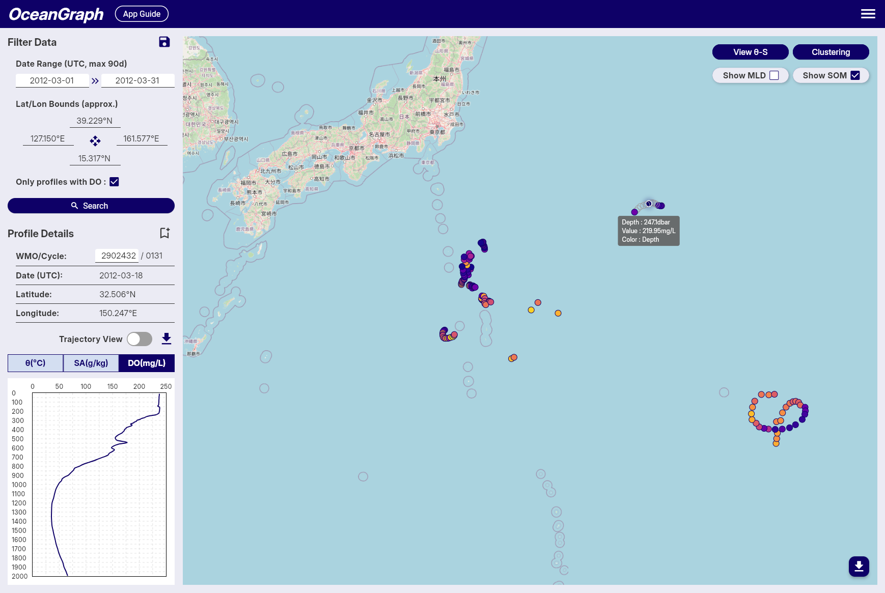
Accessing SOM
SOM display is available to signed-in users only and requires dissolved oxygen data.
- Sign in and search for profiles
- Use Only profiles with BGC if you want to focus on profiles with biogeochemical measurements
- Open MLD / SOM in the map controls and choose SOM
- Use the marker colors and tooltips to compare SOM depth and oxygen values
MLD, SOM, and mode water map overlays are mutually exclusive. Selecting SOM turns off MLD and mode water coloring. Profiles without dissolved oxygen data or a valid SOM result are rendered as no-data markers.
When Trajectory View and an oxygen section chart are open, selecting SOM also overlays an SOM line on the vertical section.
Calculation Details
-
Definition and Search Range
- When MLD is available, the SOM is defined as the local maximum of dissolved oxygen concentration found within the subsurface layer, between the mixed layer depth + 5 dbar and 300 dbar.
- When MLD is not available, the search starts at 30 dbar and extends to 300 dbar.
- If MLD is 300 dbar or deeper, SOM is not calculated for that profile.
- The very shallow layers are excluded to avoid the influence of transient surface processes and ensure the detected maximum is truly subsurface.
-
Identification of Local Maximum
- Within the specified pressure range, the oxygen profile is scanned for local maxima, defined as points where the dissolved oxygen concentration is greater than at both adjacent pressure levels.
- If multiple local maxima are present, the one with the highest oxygen concentration is selected as the SOM.
-
Fallback if No Local Maximum Exists
- If no local maximum exists within the subsurface layer (e.g., if the profile is monotonic), the single highest dissolved oxygen concentration within this range is selected as the SOM.
-
Output
- The pressure (or depth) and the corresponding dissolved oxygen concentration of the SOM are recorded for each profile.
- If no valid SOM can be identified (e.g., due to insufficient data points), the SOM is considered undefined for that observation.
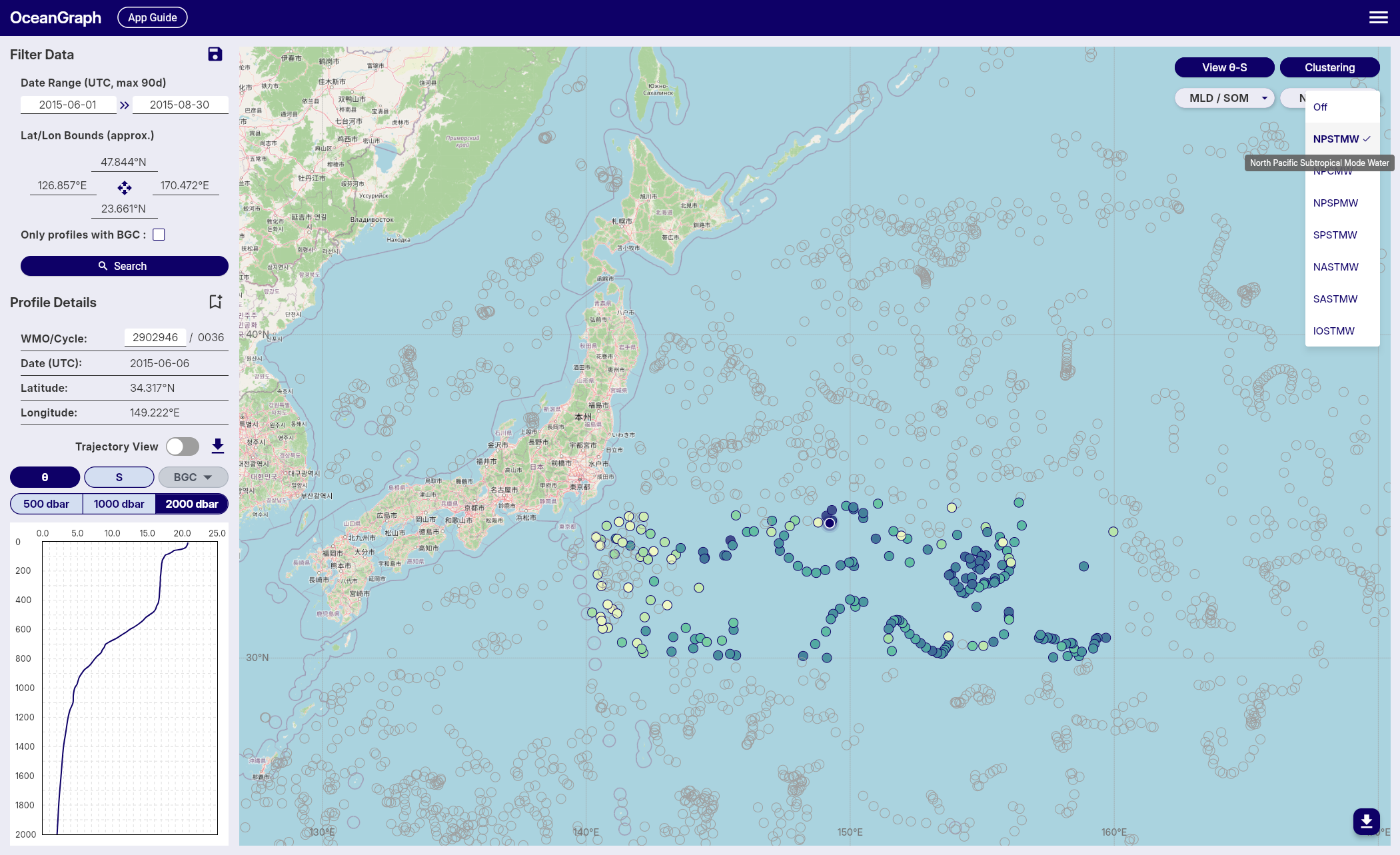
Mode Water Map Overlay
OceanGraph can color search-result map markers by profile-level mode water detection. This helps you inspect where individual profiles match a selected mode water type, and how thick the detected layer is.
This map overlay is separate from Visual Lab > Mode Waters. The map overlay works on the profiles in your current search results, while Visual Lab shows precomputed seasonal summaries and time series.
Accessing the Overlay
Mode water map overlay is available to signed-in users.
- Sign in and perform a search
- Open the Mode Water map control
- Choose one mode water type, such as NPSTMW or NASTMW
- Use marker colors and tooltips to compare detected layer thickness across profiles
The MLD / SOM and Mode Water controls are mutually exclusive. Selecting a mode water turns off MLD and SOM coloring, and selecting MLD or SOM turns off mode water coloring. Both controls include Off when you want to return to the default marker colors.
Marker Colors and Tooltips
When a mode water type is selected:
- Profiles with that mode water are colored by detected layer thickness.
- Profiles without that selected mode water are shown as no-data markers.
- The tooltip shows the selected mode water type, layer thickness, core depth, and that marker color represents thickness.
Thickness is mapped to color with the same cmocean deep colormap used for MLD map coloring. Color should be read as a relative visual cue for comparing profiles in the current result set, not as a separate classification variable.
Supported Mode Water Types
The region column reflects OceanGraph’s default advection processing scope, which searches broader areas that can include advected mode water signals.
| Short name | Full name | Region | Density range |
|---|---|---|---|
| NPSTMW | North Pacific Subtropical Mode Water | 20°N-38°N, 130°E-180° | 25.0-25.6 σθ |
| NPCMW | North Pacific Central Mode Water | 20°N-45°N, 145°E-145°W | 26.0-26.6 σθ |
| SPSTMW | South Pacific Subtropical Mode Water | 25°S-42°S, 150°E-170°W | 25.8-26.5 σθ |
| NASTMW | North Atlantic Subtropical Mode Water | 20°N-42°N, 85°W-35°W | 26.3-26.6 σθ |
| SASTMW | South Atlantic Subtropical Mode Water | 25°S-42°S, 60°W-20°E | 26.2-26.7 σθ |
| IOSTMW | Indian Ocean Subtropical Mode Water | 25°S-45°S, 20°E-70°E | 25.8-26.2 σθ |
All listed mode water types use a maximum potential vorticity threshold of 2 × 10⁻¹⁰ m⁻¹s⁻¹ and a minimum detected layer thickness of 10 m.
Detection Details
Mode water detection is calculated during OceanGraph data processing for each profile. The detection uses quality-controlled, interpolated pressure, potential temperature, and absolute salinity profiles. A profile is checked against the configured geographic bounds for each mode water type, then a continuous layer is detected using density, potential vorticity, and minimum-thickness criteria.
For each detected layer, OceanGraph records:
- Top pressure and bottom pressure in dbar
- Thickness in meters
- Core depth in meters
Core depth is defined as the midpoint of the detected layer after converting the top and bottom pressures to depth. It is not the depth of minimum potential vorticity.
A single profile can store more than one detected mode water type. The map, however, colors markers for the one type currently selected in the Mode Water control.
Interpreting No-Data Markers
A no-data marker does not necessarily mean the profile is unusable. It means the selected mode water type was not detected for that profile under OceanGraph’s current automatic criteria. Common reasons include:
- The profile is outside the selected mode water’s geographic bounds
- The density or potential vorticity criteria were not met
- The matching layer was thinner than the 10 m minimum required thickness
- The profile did not have enough valid data after quality control and interpolation
Mode water detection is intended as an exploration aid. For research-grade classification, inspect the original profile structure and apply the criteria appropriate to your study.
Visual Lab
This section contains advanced visualization tools for analyzing large-scale oceanographic trends and water mass characteristics using Argo float data.
Visual Lab is available to signed-in users from Menu > Visual Lab in the live app.
Open OceanGraph to browse Visual Lab views in the live app.
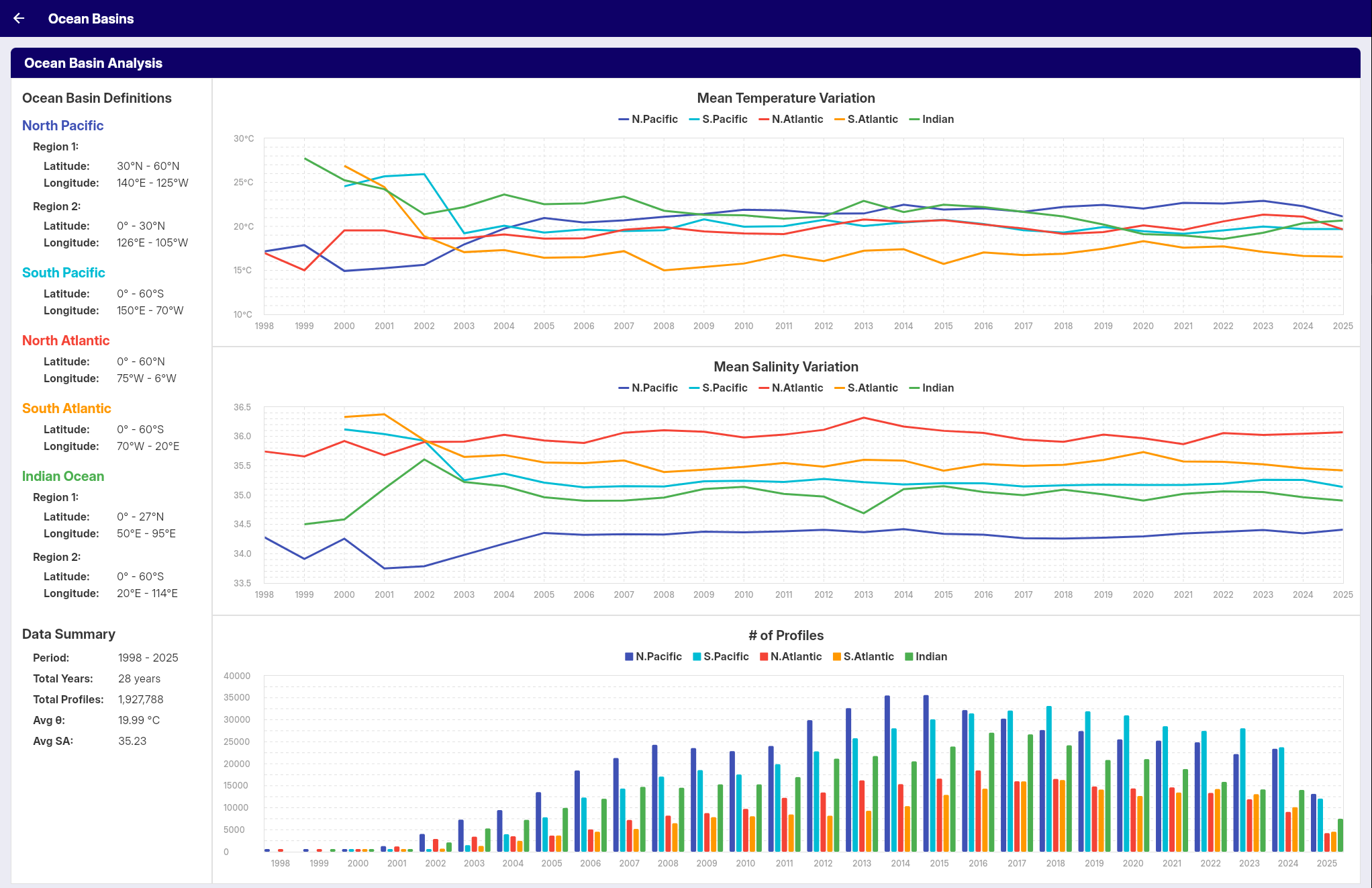
Ocean Basins visualizes time series of average temperature and salinity changes across the world’s major ocean basins (North Pacific, South Pacific, North Atlantic, South Atlantic, and Indian Ocean) from 1998 to the present. This tool helps identify long-term oceanographic trends at regional scales.
Mode Waters detects and analyzes mode water layers in Argo float profiles based on density, potential vorticity, and thickness criteria. This feature provides time series visualization of mode water thickness trends and seasonal distribution patterns.
Ocean Basins
Overview
The Ocean Basins feature provides time series visualization of average temperature and salinity changes across the world’s major ocean basins. This tool displays long-term oceanographic trends using Argo float data from 1998 to the present.
Accessing Ocean Basins
Ocean Basins is available to signed-in users.
- Sign in to OceanGraph
- Open the app menu
- Select Visual Lab > Ocean Basins
Ocean Basins Coverage
The analysis covers five major ocean basins: North Pacific, South Pacific, North Atlantic, South Atlantic, and Indian Ocean. Each basin’s data is analyzed separately to reveal regional trends.
Data Visualization
Temperature and Salinity Graphs
The feature displays two main types of time series:
- Average Temperature: Long-term trends in ocean potential temperature by basin
- Average Salinity: Long-term trends in ocean absolute salinity by basin
Data Parameters
- Temperature: Potential temperature (θ) values at 10 dbar depth
- Salinity: Absolute salinity (SA) values at 10 dbar depth
Time Period
- Coverage: 1998 to the present
- Data Source: Argo float profile measurements interpolated using the Akima method
- Temporal Resolution: Annual
Profile Count Display
The visualization includes an additional bar chart showing:
- Annual Profile Count: Number of Argo profiles used each year for each basin
This profile count chart helps users understand data density and reliability over time.
Interpretation Notes
- Early years have fewer Argo profiles than recent years, so profile counts should be checked before comparing long-term values.
- The annual averages are intended for exploratory visualization and education. Use the original Argo data and an appropriate reproducible workflow for publication-grade analysis.
Applications
This tool is useful for:
- Understanding regional ocean climate variations
- Identifying long-term trends in ocean temperature and salinity
- Comparing oceanographic changes between different basins
- Educational purposes and oceanographic research
Mode Waters
The Mode Waters feature displays the detection and time series visualization of mode water layers in Argo float profiles.
This page describes the Visual Lab view, which summarizes mode water detections by season. For coloring the markers in your current map search by profile-level mode water detection, see Mode Water Map Overlay.
This tool provides:
- Detection of mode water layers in profiles based on specified criteria
- Count of profiles containing mode water by season
- Time series visualization of mode water thickness trends
- Statistical display of thickness values (median and quartiles)
Accessing Mode Waters
Mode Waters is available to signed-in users.
- Sign in to OceanGraph
- Open the app menu
- Select Visual Lab > Mode Waters
Detection Criteria
Mode water detection uses criteria displayed on the screen (latitude/longitude bounds, density range, potential vorticity threshold, and minimum thickness).
The same profile-level detection results are also used by the map overlay. Visual Lab aggregates those detections into seasonal time series, while the map overlay shows the selected mode water on individual search-result markers.
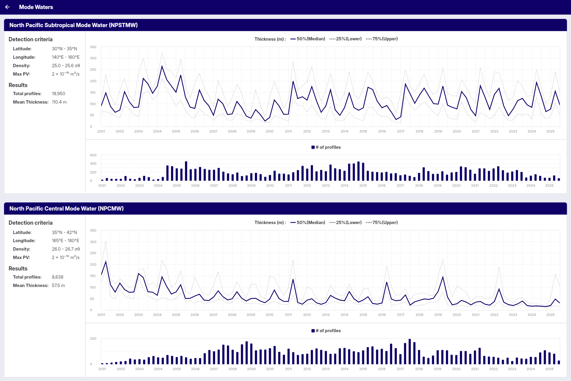
Results Display
The panel displays:
- Total Profiles: Number of profiles containing detected mode water layers
- Mean Thickness: Average of the seasonal median thickness values shown in the time series
Graphs
Time Series Graph
Displays mode water thickness over time:
- Median Thickness: 50th percentile (solid blue line)
- Lower Quartile: 25th percentile (dashed gray line)
- Upper Quartile: 75th percentile (dashed gray line)
- Time Scale: Seasonal data from 2001 onwards
Profile Count Graph
Shows the number of profiles containing mode water:
- Blue Bars: Number of profiles per season
- Time Scale: Seasonal data from 2001 onwards
Data Processing
Quality Control
The analysis applies strict quality control measures to ensure reliable results:
-
Geographic Filtering
- Only profiles within the specified target region are analyzed
- Profiles outside the geographic bounds are excluded
-
Profile Depth Requirements
- Minimum profile depth: 500 dbar (approximately 500m)
- Profiles that are too shallow are excluded from analysis
-
Data Completeness
- Minimum 10 valid data points required per profile (temperature, salinity, pressure)
- Minimum 5 valid density data points required for mode water calculation
- Minimum 3 valid data points required for potential vorticity calculation
- Profiles with insufficient temperature, salinity, or pressure data are excluded
- Missing or invalid data points are removed before analysis
- Mode water layers must be ≥10m thickness to be included in analysis
Seasonal Grouping
Data is grouped by meteorological seasons:
- Winter: December, January, February
- Spring: March, April, May
- Summer: June, July, August
- Autumn: September, October, November
Background
Mode waters are water masses characterized by weak vertical gradients in temperature and salinity, forming relatively uniform layers. They are created by deep winter mixed layers and play important roles in ocean circulation.
This feature displays basic statistics and time series of detected mode water layers in the specified region.
Analysis Lab
This section provides tools for custom analysis of oceanographic data. These features allow you to work with your own datasets and perform specialized analyses beyond the standard search and visualization capabilities.
Open OceanGraph to move between the live app and your custom analysis workflow.
Analysis Lab is available to signed-in users from Menu > Analysis Lab. The current Vertical Profiles tool is available on desktop browsers only.
Vertical Profiles allows you to upload and visualize custom vertical profile data in JSON format. This tool enables you to compare multiple profiles of temperature, salinity, dissolved oxygen, and supported BGC variables, add a note for downloaded files, and export charts. Designed for researchers and students working with Argo-format oceanographic data.
Vertical Profiles
The Vertical Profile Viewer is a feature of OceanGraph that allows you to visualize and compare vertical profiles of oceanographic data.

With this tool, you can:
- Upload one or more JSON files containing vertical profile data.
- Visualize temperature, salinity, dissolved oxygen, and supported optional BGC variables by depth.
- Add a brief note that is included in the downloaded ZIP file.
- Download profile charts, a shared legend, and the note as a ZIP file.
This feature is designed for researchers, students, and ocean enthusiasts who wish to analyze and compare their own custom oceanographic data — especially data that follows the variable structure commonly used in Argo float observations.
Access and Limits
Vertical Profiles is available to signed-in users on desktop browsers only.
- Open Menu > Analysis Lab > Vertical Profiles in the live app.
- Upload up to 30 JSON files.
- If you upload a file with the same filename as an existing uploaded file, the previous file is replaced.
- Select or deselect uploaded files to control which profiles are shown in the charts.
- Use Clear All to remove uploaded files and clear the note.
The downloaded ZIP contains one PNG file for each chart type, a shared legend image when profiles are loaded, and note.txt.
Supported JSON Format
The JSON structure used in this tool is based on the variable naming conventions of Argo float profiles. Each uploaded file must be a JSON file with the following required keys:
{
  "pressure": [ ... ],
  "potential_temperature": [ ... ],
  "absolute_salinity": [ ... ],
  "oxygen": [ ... ],
  "wmo_id": "2902447",
  "cycle_number": 17
}
"pressure": array of numbers (required, must not be empty)"potential_temperature": array of numbers (required; if non-empty, same length aspressure)"absolute_salinity": array of numbers (required; if non-empty, same length aspressure)"oxygen": array of numbers — dissolved oxygen concentration (μmol/kg) (required; if non-empty, same length aspressure)"wmo_id": string or number (required, up to 20 characters after conversion to text)"cycle_number": number (required)
Optional BGC keys can also be included:
"chlorophyll": array of numbers or nulls — chlorophyll-a (mg/m³) (same length aspressure, if present)"nitrate": array of numbers or nulls — nitrate (μmol/kg) (same length aspressure, if present)"bbp700": array of numbers or nulls — particulate backscattering at 700 nm (m⁻¹) (same length aspressure, if present)"ph": array of numbers or nulls — in-situ pH (same length aspressure, if present)"irradiance490": array of numbers or nulls — downwelling irradiance at 490 nm (W/m²/nm) (same length aspressure, if present). This key is accepted, but it is not displayed as a chart in the current interface."par": array of numbers or nulls — photosynthetically available radiation (μmol/m²/s) (same length aspressure, if present)
Any additional keys will be ignored. Files that do not follow the required structure or fail validation will be skipped during upload.
Articles
This page serves as the main index for OceanGraph-related articles.
Open OceanGraph to explore real Argo data after reading these articles.
Getting Started with Argo
- What is Argo Float? A Complete Guide to Ocean Observation Data
- How to Read Argo Float Data for Beginners (What to Look at First)
- Finding Argo Float Profiles by Location, Time, and WMO ID
- Argo NetCDF Format Explained for Beginners
Reading Ocean Structure
- Ocean Temperature and Salinity Profiles Explained
- T-S Diagrams in Oceanography Explained (With Examples)
- Salinity and Temperature in the Ocean Explained
Biogeochemical Argo
Visualization and Workflow
- Ocean Data Visualization: Methods, Examples, and Tools
- Time-Series Vertical Sections in Oceanography Explained (With Argo Examples)
- Visualizing Argo Float Data Without Python (Step-by-Step Guide)
- Making a T-S Diagram: Python vs Interactive Tools
What is Argo Float? A Complete Guide to Ocean Observation Data
If you are new to oceanography, one of the first terms you will encounter is Argo float. Argo floats are autonomous instruments that drift through the ocean, dive below the surface, and return measurements that help scientists understand how the ocean changes over time.
They matter because ocean conditions are not static. Temperature, salinity, oxygen, and other properties vary with depth, season, and location. To understand the real structure of the ocean, you need more than a surface map. You need vertical profiles collected repeatedly across the globe. That is exactly what Argo provides.
This guide explains what an Argo float is, how it works, what kind of data it produces, why Argo data is so important, and how to start exploring real Argo profiles without writing Python code.
What Is an Argo Float?
An Argo float is an autonomous profiling float used for ocean observation. It is part of the International Argo Program, a global effort to collect consistent, repeat observations of the upper and middle ocean.
Each float spends most of its time below the sea surface. It drifts with ocean currents, dives to a target depth, then rises back toward the surface while measuring the water column. After surfacing, it sends its observations through satellite communication before beginning the next cycle.
In simple terms:
- A float is the instrument
- A profile is one vertical set of measurements
- A cycle is one repeat of drifting, diving, profiling, and transmitting
Argo transformed ocean observation because it made subsurface measurements more routine, global, and comparable. Before Argo, many measurements depended on ship campaigns, which were valuable but limited in time and space.
Why Argo Floats Matter
Argo floats fill a major observational gap between two older approaches:
- Satellites give broad coverage, but they mainly observe the ocean surface
- Ships can measure the water column directly, but only along limited routes and schedules
Argo floats provide a third kind of observing system: repeated subsurface measurements across wide areas of the ocean. That makes them useful for:
- Tracking changes in temperature and salinity
- Understanding seasonal and regional ocean structure
- Studying water masses and mixing
- Monitoring ocean heat content
- Supporting climate research and model validation
For students and early-career researchers, Argo is often the easiest entry point into large-scale ocean observation data because the measurements are physically meaningful and organized as profiles.
How Does an Argo Float Work?
A typical Argo float follows a repeating cycle:
- It starts near the surface after transmitting data.
- It sinks to a parking depth, often around 1,000 meters.
- It drifts with currents for several days.
- It then sinks deeper, often to around 2,000 meters.
- It rises toward the surface while recording measurements through the water column.
- Once at the surface, it sends the profile and position data by satellite.
- The cycle repeats.
This repeated behavior is why Argo data is so powerful. A single float does not just observe one place once. It creates a time series of vertical ocean profiles along a drifting path.
What Does an Argo Float Measure?
The core Argo system is best known for measuring:
- Pressure
- Temperature
- Salinity
In practice, salinity is derived from conductivity, temperature, and pressure measurements. These variables are enough to describe a large part of the ocean’s physical structure.
Some Argo floats carry additional sensors, especially in biogeochemical programs. Depending on the float, you may also encounter:
- Dissolved oxygen
- Chlorophyll-related optical measurements
- Nitrate
- pH
- Particle backscatter
- Light-related variables such as irradiance
This is why Argo data is useful across different levels of oceanography. A beginner may start with temperature and salinity profiles, while a more advanced user may move into oxygen, productivity, or water-mass analysis.
What Does Argo Data Look Like?
Argo data is usually organized around floats and cycles.
Some of the most common concepts are:
| Term | Meaning |
|---|---|
| WMO ID | The identifier for a specific float |
| Cycle number | The sequence number for one profile event |
| Profile | A vertical set of observations from one ascent |
| Trajectory | The float positions through time |
| Pressure levels | The sampled points through the water column |
If you open an Argo data file, you will usually see arrays of values for pressure, temperature, salinity, time, location, quality flags, and metadata. That structure is powerful, but it can also be intimidating if you are new to NetCDF files or oceanographic naming conventions.
For many users, the first practical views of Argo data are not the raw files themselves but visual products such as:
- Temperature vs depth
- Salinity vs depth
- Oxygen vs depth
- Float trajectory maps
- Temperature-salinity or theta-salinity diagrams
Those visualizations are often the fastest way to build intuition before moving into full Argo float data analysis.
Core Argo, BGC Argo, and Deep Argo
You may also hear about several related Argo categories:
- Core Argo focuses mainly on physical variables such as temperature and salinity
- BGC Argo adds biogeochemical sensors such as oxygen, nitrate, pH, or optical variables
- Deep Argo extends observations deeper than the standard core profiling range
You do not need to master all of these on day one. The important first step is understanding that Argo is not just one data product. It is a broader observing system with related profile types and use cases.
How Beginners Should Read Argo Profiles
If you are just starting, the best approach is to read Argo data in layers.
1. Start with place and time
Before looking at any profile, check:
- Where was the float?
- When was the profile taken?
- Is it one profile or part of a sequence?
This gives you geographic and seasonal context.
2. Look at one variable against depth
A temperature profile can show you:
- Surface warming
- Mixed layers
- Sharp gradients
- Deep stability
A salinity profile can show you:
- Fresh surface layers
- Salty subsurface water
- Vertical structure associated with different water masses
3. Compare multiple cycles
One profile is useful. A sequence of profiles is much better. Comparing nearby cycles helps you see how the upper ocean changes in time and whether a feature is persistent or temporary.
4. Use a T-S diagram to understand water masses
A depth profile shows vertical structure. A T-S diagram shows how temperature and salinity relate to each other. Both views matter. If you want to understand water-mass structure, mixing, or the identity of different layers, a T-S view becomes especially useful.
OceanGraph includes a dedicated guide for θ-S Diagram, which is a good next step after learning the basics.
Why Argo Data Often Feels Hard at First
Argo is conceptually simple, but working with the data can still feel harder than expected.
Common reasons include:
- Raw files are often distributed in NetCDF format
- Variable names and metadata are not always beginner-friendly
- Quality control flags need to be interpreted correctly
- One float can have many cycles, files, and derived products
- Plotting useful figures often requires code before you fully understand the data
This creates a common frustration loop:
- You want to understand Argo data
- You download files
- You spend most of your time handling format and plotting
- You still have not built intuition about the ocean structure itself
That is exactly why visual exploration matters.
A Better First Step: Explore Before You Code
Before writing scripts, it helps to answer simpler questions first:
- What does a real Argo profile look like?
- How does one float change over time?
- What does a water mass pattern look like in profile space?
- Which profiles are worth deeper analysis later?
OceanGraph is designed for that stage of work. Instead of starting with file parsing, you can start with interpretation.
With OceanGraph, you can:
- Search Argo profiles by region, time, and WMO ID
- Inspect trajectories and time-series sections
- Explore vertical profiles interactively
- View θ-S diagrams to understand water-mass structure
Useful starting points:
Try Real Argo Data in OceanGraph
If your goal is not just to learn the definition of an Argo float but to actually see ocean observation data, OceanGraph is the next step.
Try with real Argo data -> OceanGraph
Explore profiles interactively
OceanGraph helps bridge the gap between reading about Argo and doing something useful with Argo float data. You can build intuition first, then move to deeper analysis once you know which profiles, regions, or patterns matter.
Frequently Asked Questions
Is an Argo float the same as a buoy?
No. A surface buoy usually stays near the surface or at a fixed location. An Argo float is designed to move vertically through the water column and drift between cycles.
Does every Argo float measure the same variables?
No. Core Argo floats mainly provide physical measurements such as temperature and salinity. Other programs add sensors for oxygen, nitrate, pH, optics, and related variables.
What is the difference between a float and a profile?
A float is the instrument. A profile is one set of vertical measurements collected during a single ascent.
Do I need Python to start using Argo data?
Not necessarily. Python becomes useful for custom analysis, but it is not the best first step for everyone. Many beginners learn faster by exploring trajectories, profiles, and T-S structure visually first.
Conclusion
Argo floats are one of the most important tools in modern oceanography because they make subsurface ocean observation data available at global scale and repeated over time. If you want to understand ocean structure, water masses, seasonal variability, or profile-based analysis, Argo is a foundational dataset.
The fastest way to begin is not to memorize file formats. It is to look at real profiles, connect them to place and time, and build intuition from the data itself. That is where OceanGraph can help.
How to Read Argo Float Data for Beginners (What to Look at First)
If you are new to Argo float data, the first obstacle is often not oceanography. It is figuring out what you are looking at. A raw Argo profile contains measurements, metadata, quality information, and cycle context, but when you first open the data it is not obvious which parts matter most.
That is why many beginners ask a practical question before anything else: how do you actually read Argo data? Not how do you download it, and not how do you code with it, but what should you look at first so the profile starts to make sense.
This guide explains how to read Argo float data step by step. It covers the basic fields, the main variables, the most common beginner mistakes, and a simpler workflow for exploring real Argo profiles in OceanGraph before you write Python.
If you are completely new to Argo itself, start with What is Argo Float? A Complete Guide to Ocean Observation Data.
Why Argo Data Feels Hard When You First Open It
Argo data is physically meaningful, but it is not always visually obvious.
When you first encounter a profile, you may see:
- A WMO ID
- A cycle number
- Latitude and longitude
- Time information
- Arrays of pressure, temperature, and salinity
- Quality flags and metadata fields
All of that is useful, but beginners often see it in the wrong order. They start from file structure or variable names instead of starting from the scientific question: where was this profile collected, when was it measured, and what does the water column look like?
That is the key shift. Argo data becomes easier when you read it as an observation of ocean structure, not as a file format problem.
What Argo Float Data Usually Contains
At the most basic level, one Argo profile combines:
- Context about the observation
- Measurements through the water column
- Metadata that helps you interpret the measurements correctly
The most common fields beginners need to understand are:
| Field | What it tells you |
|---|---|
| WMO ID | Which float produced the observation |
| Cycle number | Which profile event this is in the float’s sequence |
| Date and time | When the profile was taken |
| Latitude and longitude | Where the float surfaced or reported |
| Pressure | The vertical sampling coordinate |
| Temperature | Thermal structure of the water column |
| Salinity | Salt content and water-mass information |
| Quality flags | Whether a value passed quality control checks |
If you want a broader explanation of how floats, profiles, and cycles relate to each other, What is Argo Float? A Complete Guide to Ocean Observation Data is the best starting point.
The important practical point is this: you do not need to understand every metadata field before you can start reading a profile well. You need only enough context to interpret the measurement in place and time.
The First Things to Check Before Reading a Profile
Before focusing on the graph itself, check a few basics first.
1. Start with location and date
Ocean structure depends strongly on where and when the profile was taken.
A profile from the subtropical North Pacific in summer should not be interpreted the same way as one from the Southern Ocean in winter. Even before looking at the line shape, ask:
- Which ocean basin is this profile from?
- Is it coastal or open ocean?
- What season does the date imply?
- Is this a region where strong stratification, freshening, or deep mixing is common?
These questions keep you from over-interpreting the profile in isolation.
If you want to inspect this context directly before reading the graph, OceanGraph’s Search and Bookmark workflow is useful because it keeps date, location, WMO ID, and cycle information visible while you explore.
2. Check cycle number and profile context
One of the biggest beginner mistakes is treating a single profile as if it were the whole story.
Argo floats collect repeated profiles over time. That means one profile is usually part of a sequence. The cycle number helps you place the observation in that sequence.
This matters because:
- A feature may be persistent across many cycles
- A surface anomaly may appear only for one short period
- Deep structure may remain stable while upper-ocean structure changes
If you compare one cycle with nearby cycles from the same float, interpretation gets much easier. The best first question is often not “what is this line?” but “does this line look similar to the previous and next profiles?”
3. See which variables are available
Not every Argo profile contains the same variables.
Many profiles include the core physical variables:
- Pressure
- Temperature or potential temperature
- Salinity or absolute salinity
Some also include biogeochemical measurements such as:
- Dissolved oxygen
- Chlorophyll-related optical variables
- Nitrate
- pH
For beginners, it is usually best to start with temperature and salinity because they describe the basic physical structure of the water column. Once you understand those, the rest of the profile becomes easier to place in context.
How to Read the Main Variables
Once you know the profile context, move to the measurements themselves.
Temperature
A temperature profile is often the easiest place to begin.
Look for:
- A warm or cool surface layer
- A relatively uniform upper layer
- A sharp gradient below the surface
- Stable deep values
These patterns help you identify whether the upper ocean is strongly stratified, recently mixed, or transitioning between seasonal states.
When reading temperature, focus first on the shape of the profile rather than any single number. A single surface value matters less than whether the profile shows a shallow warm layer, a strong thermocline, or a gradual transition.
If you want a dedicated guide to profile interpretation, see Ocean Temperature and Salinity Profiles Explained.
Salinity
Salinity is often the variable beginners underestimate at first.
Temperature is intuitive because people already think in warm and cold. Salinity is less familiar, but in oceanography it is equally important because it helps distinguish water masses and contributes to density.
A salinity profile can show:
- Surface freshening from rainfall, runoff, or ice melt
- Surface salinification from evaporation
- A halocline or strong salinity gradient
- Subsurface salinity maxima or minima
Two profiles with similar temperature structure may still represent very different water masses if their salinity differs. That is why a temperature-only view is never enough for serious interpretation.
Pressure and depth
Argo profiles are usually organized by pressure, not literal geometric depth.
In many practical cases, pressure is close enough to depth to support intuitive interpretation, especially for beginners. But they are not identical, and it is better to think of pressure as the actual measured vertical coordinate.
For reading a profile, the practical lesson is simple:
- Higher pressure means deeper water
- Near-surface values are at low pressure
- Deep values are at high pressure
Do not get stuck on the conversion at the start. Focus on the vertical structure and relative changes first.
Quality flags and missing values
Another thing that confuses beginners is that some points may be missing, filtered, or flagged.
Quality information matters because oceanographic data is not just about plotting every number you see. Some values may need caution, especially in derived or biogeochemical fields.
You do not have to become a quality-control expert on day one, but you should remember:
- Missing points do not automatically mean the profile is useless
- One suspicious point should not outweigh the shape of the whole profile
- Apparent spikes may reflect data issues rather than physical structure
This is one reason visual inspection is so helpful. It is often easier to notice odd structure on a graph than in a table of numbers.
A Simple Example: Reading One Argo Profile Step by Step
Imagine you open one Argo profile from a subtropical region in late summer.
A practical reading sequence would look like this:
- Check the location and date.
- Confirm which float and cycle you are looking at.
- Open the temperature profile.
- Look for the surface layer, the main gradient, and the deep structure.
- Open the salinity profile and ask whether it reinforces or changes your first interpretation.
- Compare with nearby cycles or nearby profiles.
- Use a T-S style view if you want to understand the water-mass relationship more clearly.
Suppose the temperature profile shows:
- Warm surface water
- A clear thermocline below it
- Relatively stable deeper values
Then the salinity profile shows:
- Slightly fresher surface water
- A saltier subsurface layer
- More stable deep salinity
That already tells you much more than “this file contains numbers.” It suggests a stratified upper ocean, surface modification processes, and a subsurface layer with distinct water properties.
The next useful step is not necessarily more code. It is often comparison.
If you compare two nearby cycles and see that the deep structure is stable while the surface layer changes, you learn something physically meaningful about variability. If you open a θ-S view and see a compact deep-water cluster plus a broader surface spread, that interpretation becomes even stronger.
OceanGraph supports this kind of workflow with:
What Beginners Often Misread
Even when the graph is visible, a few mistakes come up repeatedly.
Confusing pressure with depth
Pressure is the profile coordinate you will most often see. It is fine to read it intuitively as “deeper downward,” but do not assume the label is literally depth if the dataset says pressure.
Looking at one point instead of the profile shape
A profile is not a collection of isolated numbers. It is a vertical structure.
If you focus on one value instead of the shape, you can miss:
- The mixed layer
- The main gradient zone
- Subsurface extrema
- Whether the deep water is uniform or changing
Ignoring data quality information
Not every value deserves the same confidence. If the shape looks strange, especially in a small part of the profile, consider that data quality may be part of the explanation.
The safest beginner habit is to trust the broad structure first and treat isolated odd points with caution.
The Traditional Workflow: Download, Decode, Then Plot
A common Argo workflow looks like this:
- Download NetCDF files
- Inspect variable names and metadata
- Decide which arrays matter
- Handle quality flags
- Write code to plot temperature and salinity
- Repeat the process for the next profile
That workflow is valid for research, but it can be a poor first experience for beginners. The problem is not that coding is wrong. The problem is that it forces you to solve a software workflow before you have built any intuition about the ocean structure.
This is exactly why many people end up searching for simpler paths such as Visualizing Argo Float Data Without Python (Step-by-Step Guide).
A Better First Step: Explore Argo Profiles Interactively
If your goal is to read Argo data rather than automate it immediately, interactive exploration is often the better first step.
OceanGraph helps because it keeps the interpretation workflow in the right order:
- Search by region, date, and WMO ID
- Check profile context
- Open the vertical profile
- Compare multiple observations
- Use a θ-S diagram when you need water-mass interpretation
That lets you learn the data structure through actual examples instead of through file parsing alone.
Good follow-up pages after this article are:
- Ocean Temperature and Salinity Profiles Explained
- T-S Diagrams in Oceanography Explained (With Examples)
- Visualizing Argo Float Data Without Python (Step-by-Step Guide)
- Vertical Profiles
Try Real Argo Data in OceanGraph
If you want to move from “I know the field names” to “I can actually read the profile,” the next useful step is to open real data and compare it visually.
Try with real Argo data -> OceanGraph
Explore profiles interactively
OceanGraph helps you build intuition about Argo profiles before you invest time in a heavier coding workflow.
Frequently Asked Questions
What should I check first in an Argo profile?
Start with location, date, float ID, and cycle number. That gives the profile context before you interpret the graph itself.
Is pressure the same as depth?
Not exactly. Pressure is the measured vertical coordinate used in many ocean datasets. For beginner interpretation, it is usually fine to think of higher pressure as deeper water.
What variables should I read first?
Start with temperature and salinity. They provide the clearest first view of physical ocean structure and water-mass differences.
Do I need to understand NetCDF before I can read Argo data?
No. NetCDF becomes useful when you want custom processing, but it does not have to be your first step if your immediate goal is interpretation.
What should I read after this guide?
The best next steps are Ocean Temperature and Salinity Profiles Explained and T-S Diagrams in Oceanography Explained (With Examples).
Conclusion
Reading Argo float data becomes much easier when you stop treating it as a file first and start treating it as an observation of ocean structure. The most useful beginner workflow is simple: check the profile context, read temperature and salinity against pressure, compare nearby observations, and only then worry about heavier technical steps.
That is where OceanGraph becomes useful. It lets you see real Argo data in the order that supports understanding first.
Finding Argo Float Profiles by Location, Time, and WMO ID
When people first work with Argo float data, one of the hardest steps is not reading the profile. It is finding the right profile in the first place.
Sometimes the question is regional: you want all profiles in one area during one season. Sometimes it is platform-centered: you already know a float’s WMO ID and want to follow that float across multiple cycles. Sometimes it is variable-centered: you need only profiles that include dissolved oxygen.
This guide explains the practical logic of finding Argo float profiles. It covers the difference between floats and profiles, when to search by location or by WMO ID, common mistakes, and how to explore results in OceanGraph before downloading files.
If you are completely new to the Argo system itself, start with What is Argo Float? A Complete Guide to Ocean Observation Data.
Why Finding the Right Profile Is Harder Than It Sounds
Argo is a global observing system, which means the data is rich but also easy to search in the wrong way.
Beginners often know the scientific question they care about, but not yet the search unit that matches it.
Typical starting questions sound like this:
- I want profiles from one ocean region during one month
- I want to track one float over time
- I want only profiles that include oxygen
- I want to compare several nearby profiles before coding
Those are good questions, but they point to different search strategies. The most useful first step is to decide whether you are trying to find:
- A set of profiles from a region and time window
- A single float identified by WMO ID
- A subset of profiles with a particular variable such as dissolved oxygen
Once that is clear, searching becomes much easier.
Start with the Search Units: Float, Profile, Cycle, and WMO ID
Before searching, it helps to keep four terms separate.
| Term | What it means | Why it matters for search |
|---|---|---|
| Float | The physical Argo instrument drifting and profiling over time | One float can produce many profiles |
| Profile | One vertical observation through the water column | This is usually the actual unit you compare |
| Cycle | One sampling event in the float’s sequence | Helps place the profile in time order |
| WMO ID | The identifier assigned to a float | Useful when you already know which float you want |
The key practical point is this: searching by WMO ID does not usually return one profile. It returns the sequence of profiles from one float.
That distinction matters because many beginners search for a float when they are really trying to find one profile, or they search for a region when they actually want the repeated history of one known float.
If you want a broader explanation of how these pieces fit together, How to Read Argo Float Data for Beginners (What to Look at First) is a good next step.
Three Practical Ways to Search Argo Data
Most Argo searches fall into three patterns.
1. Search by location and date when the question is regional
Use a geographic search when your question begins with a place or season.
Examples:
- What profiles are available in the subtropical North Pacific this month?
- Are there profiles near a frontal region during winter?
- What does the water column look like in this basin during a given period?
This type of search is best when you do not care which float collected the data yet. You care first about where and when.
In OceanGraph, this means starting with:
- A date range
- Geographic bounds set on the map
- The result markers that show which profiles match
The search workflow is documented here:
One useful habit is to start with a window that is broad enough to show what is available, then narrow after you see the result distribution.
2. Search by WMO ID when you want one float’s history
Use a WMO search when you already know the float identifier and want direct access to its observation sequence.
This is useful when you want to:
- Follow one float across many cycles
- Compare early and late observations from the same platform
- Revisit a float cited in a paper, class, or discussion
- Move quickly from a known ID to profile details
WMO search is efficient because it removes the uncertainty of regional browsing. Instead of asking “what is in this area?” you ask “show me this float.”
That is often the fastest route into:
- Cycle-by-cycle comparison
- Trajectory interpretation
- Time-series vertical sections
3. Filter for BGC data when the question is biogeochemical
Not every Argo profile includes the same variables.
If your question is about biogeochemical measurements, you should not start with all profiles and inspect them one by one. It is better to filter for profiles that include BGC data first.
OceanGraph includes an Only profiles with BGC option in the search panel. It returns profiles that include at least one supported BGC parameter, such as dissolved oxygen, chlorophyll, nitrate, backscattering, pH, downwelling irradiance at 490 nm, or PAR. That is useful when you want to:
- Focus on BGC-related profiles
- Avoid wasting time on core-only floats
- Find profiles that are more likely to contain the biogeochemical variable you need
If oxygen is your main goal, use the BGC filter first and then confirm that the selected profile includes dissolved oxygen. The natural next article is Dissolved Oxygen Profiles in BGC Argo Explained.
A Simple Workflow for Finding Useful Profiles
A practical beginner workflow looks like this:
- Start with a geographic area and date window if the question is regional.
- Look at the result markers before deciding which profile matters.
- Open profile details and inspect the WMO ID, cycle number, date, latitude, and longitude.
- Switch to WMO ID search if one float becomes especially relevant.
- Add the BGC filter if the question is biogeochemical.
- Save the search or bookmark key profiles if you are signed in.
This order is useful because it keeps the search tied to scientific context.
A few details are easy to overlook:
- OceanGraph shows profile dates in UTC
- WMO search returns all profiles for that float
- Saved searches and bookmarked profiles are available to signed-in users
Once you have found good candidates, the next step is usually not another search. It is reading the actual profile or comparing several of them. Visualizing Argo Float Data Without Python (Step-by-Step Guide) covers that workflow.
What People Often Get Wrong
A few search mistakes come up repeatedly.
Searching too narrowly too early
If you start with a very small region and a very short time window, you may conclude that “there is no data” when the real problem is only that the search was too restrictive.
A broader first pass helps you understand the data density before you narrow to a specific case.
Confusing float selection with profile selection
A float is not the same thing as a profile.
If you search by WMO ID, you are usually asking for an observation history, not one single measurement. You still need to decide which cycle or profile is relevant to your question.
Ignoring time context
Two profiles from the same place can mean different things if they were measured in different seasons or years.
That is why date is not just metadata. It is part of the interpretation.
Forgetting variable availability
Many learners search widely, then realize too late that the matched profiles do not contain the variable they actually need.
If the question involves oxygen or another BGC variable, use the BGC filter from the beginning, then confirm the specific variable in the selected profile.
The Traditional Workflow: Catalogs, File Names, Then Manual Checking
A common Argo workflow looks like this:
- Browse catalogs or download files from a data portal
- Open file names or metadata records
- Check which float or cycle each record represents
- Inspect whether the target variable is present
- Download several candidates
- Open them locally before deciding which ones are worth plotting
That workflow is valid, but it can be slow when your immediate problem is simply finding the right profiles.
The friction is even higher if you are also new to NetCDF structure. If that is your current barrier, Argo NetCDF Format Explained for Beginners can help.
A Better First Step: Search Interactively Before You Download
If your goal is to identify useful profiles quickly, interactive search is usually the better first step.
OceanGraph helps because it keeps the discovery workflow simple:
- Search by region and date
- Enter a WMO ID for direct access to one float
- Filter for BGC data when needed
- Inspect WMO ID, cycle number, date, and location together
- Save searches or bookmark profiles for later review
That means you can answer the practical question first: which profiles are actually worth my attention?
Then, once the interesting profiles are clear, you can move on to:
- How to Read Argo Float Data for Beginners (What to Look at First)
- Ocean Temperature and Salinity Profiles Explained
- Visualizing Argo Float Data Without Python (Step-by-Step Guide)
Find Real Argo Profiles in OceanGraph
If you want to move from vague profile hunting to a clear search workflow, OceanGraph is the direct next step.
Try with real Argo data -> OceanGraph
Explore profiles interactively
OceanGraph makes it easier to search by place, time, WMO ID, and BGC data availability before you commit to a heavier workflow.
Frequently Asked Questions
What is a WMO ID in Argo data?
It is the identifier for a specific Argo float. Searching by WMO ID is the fastest way to retrieve the sequence of profiles from one known float.
Should I search by float or by profile?
Search by float when you want the observation history of one platform. Search by region and date when you first need to discover which profiles are available.
Can I search only for BGC profiles?
Yes. OceanGraph includes a BGC filter so you can restrict the results to profiles that include at least one supported BGC parameter. It is not a DO-only filter, so confirm whether a selected profile includes dissolved oxygen when oxygen is required.
Why did my regional search return very few profiles?
The most common reasons are that the time window is too short, the region is too small, or the target variable filter is too restrictive.
Do I need to download NetCDF files before I can search effectively?
No. It is often better to identify useful profiles first, then decide which files are worth deeper analysis later.
Conclusion
Finding Argo float profiles becomes much easier once you separate regional search, WMO-based search, and variable-based filtering. The hardest part for beginners is usually not the data itself. It is choosing the right search unit.
For many workflows, the fastest path is to search interactively first, identify the profiles that matter, and only then move to plotting or coding. That is where OceanGraph is most useful.
Argo NetCDF Format Explained for Beginners
If you have downloaded Argo data and opened your first .nc file, the experience is often confusing. You expected ocean profiles. Instead, you got a long list of variables, dimensions, metadata fields, and quality-control flags.
That is why so many beginners search for an explanation of the Argo NetCDF format. The challenge is usually not whether the data exists. It is understanding how the file is organized and which parts matter first.
This guide explains what NetCDF is, how Argo profile files are typically structured, which variables you should inspect first, what beginners often misunderstand, and how to use OceanGraph to understand the data before building a full coding workflow.
If you want a profile-centered overview before the file-format details, start with How to Read Argo Float Data for Beginners (What to Look at First).
What Is NetCDF?
NetCDF stands for Network Common Data Form. It is a file format widely used for scientific data, especially when the data includes multiple variables, metadata, and dimensions such as time, depth, latitude, and longitude.
NetCDF is common in oceanography because it can store:
- Measurement arrays
- Coordinates
- Units
- Metadata
- Quality information
- Multiple dimensions in one file
That makes it powerful, but not always beginner-friendly.
When you open a NetCDF file, you do not see a narrative explanation of the observation. You see a data structure. Your first task is to translate that structure into a scientific question.
Why Argo Uses NetCDF
Argo data is more than a single column of temperature values.
A profile can include:
- Float identity
- Cycle information
- Position
- Time
- Pressure levels
- Temperature and salinity
- Quality flags
- Additional variables such as oxygen in some cases
NetCDF is useful because it keeps those components together in a consistent machine-readable format.
The downside is that the file is optimized for storage and exchange, not for beginner interpretation.
How to Think About an Argo File
The best way to understand an Argo NetCDF file is not to memorize every variable name. It is to think in layers.
At a high level, one Argo profile file usually combines:
- Observation context
- Measurement arrays
- Quality and status information
- Metadata about the platform or processing
If you read the file in that order, it becomes easier.
1. Observation Context: What Profile Am I Looking At?
Before worrying about the measurement arrays, identify the observation itself.
The first questions are:
- Which float produced this profile?
- Which cycle is it?
- When was it taken?
- Where was it reported?
Common fields you will often encounter include:
PLATFORM_NUMBERfor the float identityCYCLE_NUMBERfor the profile sequenceJULDfor time informationLATITUDELONGITUDE
The exact combination can vary depending on file type and processing level, but the goal stays the same: place the profile in time and space before interpreting the measurements.
This is important because Argo data is easiest to understand as an observation event, not as a list of variable names.
2. Measurement Arrays: What Was Observed Through the Water Column?
Once you know the profile context, move to the measurement arrays.
In many core Argo profile files, the most important variables are:
PRESTEMPPSAL
These usually represent:
- Pressure
- Temperature
- Practical salinity
Some files also include adjusted versions such as:
PRES_ADJUSTEDTEMP_ADJUSTEDPSAL_ADJUSTED
The practical beginner takeaway is simple:
- Start by identifying the main profile variables
- Check whether adjusted versions are present
- Do not try to interpret every variable at once
If you are using biogeochemical Argo data, you may also encounter variables such as dissolved oxygen or other sensor products. But for first-pass understanding, pressure, temperature, and salinity are usually enough.
3. Quality Information: Can I Trust Every Value Equally?
One reason Argo NetCDF files feel complicated is that they do not store measurements alone. They also store quality information.
You may see fields such as:
PRES_QCTEMP_QCPSAL_QCPOSITION_QC
The exact interpretation depends on the Argo conventions for the file, but the general point is consistent: not every value should be treated identically without checking its quality status.
For beginners, a useful rule is:
- Do not panic when you see QC fields
- Remember that quality information is part of responsible interpretation
- Focus first on recognizing the overall profile structure
A questionable point or missing value does not automatically make the whole profile unusable.
4. Dimensions: Why Do the Arrays Have Different Shapes?
Another common point of confusion is the array structure.
Argo NetCDF files often organize values using dimensions such as:
- Number of profiles
- Number of vertical levels
- Number of parameters
That means some variables look like one-dimensional arrays, while others are stored across more than one dimension.
Beginners often get stuck here because they expect the file to behave like a simple spreadsheet. But the data is hierarchical:
- A float can have profiles
- A profile can have many depth or pressure levels
- Each level can have several measured variables
You do not need to master the full dimensional design immediately. What matters first is understanding which array corresponds to the water-column observations you want to inspect.
The First Variables to Check
If you open an Argo NetCDF file and want the fastest path to understanding, inspect the data in this order:
- Float identity
- Cycle number
- Time
- Latitude and longitude
- Pressure
- Temperature
- Salinity
- Quality-control fields
This order matches the scientific workflow better than opening the file alphabetically.
It answers:
- What is this observation?
- Where and when did it happen?
- What does the water column look like?
- Are there any quality issues I need to keep in mind?
Raw vs Adjusted Variables
One detail that often confuses beginners is the presence of both raw-looking variables and adjusted variables.
You may see a pair such as:
TEMPTEMP_ADJUSTED
or
PSALPSAL_ADJUSTED
The exact use depends on the data product and processing context, but the practical point is that Argo files may contain both measurement values and versions that reflect later calibration or correction workflows.
For a beginner, the safest approach is:
- Notice whether adjusted variables exist
- Check the file documentation or workflow you are following
- Avoid mixing variables casually without knowing why
You do not need to become an expert in processing conventions on day one. You do need to recognize that the distinction exists.
Common Beginner Mistakes
Most problems come from reading the file in the wrong order.
Starting with file structure instead of observation context
If you begin with obscure variables and dimensions, the file feels abstract. Start with float, cycle, time, and location.
Treating one profile as the whole float
An Argo float produces many cycles. A single profile is one observation in a sequence, not the whole story.
Ignoring quality fields completely
You do not need to decode everything immediately, but quality information is part of proper data use.
Assuming pressure is just a cosmetic coordinate
Pressure is the core vertical coordinate in the profile and determines how you read the water-column structure.
Trying to understand everything before visualizing anything
This is one of the biggest workflow mistakes. A profile often becomes clearer once you see it plotted.
Example: A Better Way to Read an Argo NetCDF File
Suppose you open a profile file and see dozens of variable names.
A better beginner workflow is:
- Identify the float and cycle.
- Check the date and location.
- Find the pressure, temperature, and salinity arrays.
- Confirm whether adjusted versions are present.
- Look at quality fields only after you understand the basic profile structure.
- Plot or inspect the profile visually.
This sequence turns a confusing NetCDF file into a readable ocean observation.
The Traditional Workflow: Python First
Many people approach Argo NetCDF files by opening them directly in Python with a scientific library and then building plots from scratch.
That is a valid workflow, but beginners often hit several friction points:
- NetCDF feels unfamiliar
- Variable names are not self-explanatory at first
- Quality fields interrupt the first reading
- You may debug indexing before you understand the water column
- Comparing several files still takes setup
If your first goal is understanding rather than automation, this can be heavier than necessary.
A Better First Step: Understand the Observation Before the File
OceanGraph is useful because it lets you approach Argo data from the observation side first.
Instead of beginning with file parsing, you can:
- Search real profiles by region, time, and WMO ID
- Inspect the profile context directly
- Open vertical profiles immediately
- Compare several observations before deciding what to code later
Useful follow-up pages are:
- Search and Bookmark
- Vertical Profiles
- Visualizing Argo Float Data Without Python (Step-by-Step Guide)
Once you already know which float, cycle, or pattern matters, the NetCDF file becomes much easier to approach.
Explore Argo Data Before You Parse the File
If you want to reduce file-format friction and understand what the data actually represents first, OceanGraph is a practical place to start.
Try with real Argo data -> OceanGraph
Explore profiles interactively
OceanGraph helps bridge the gap between opening an Argo NetCDF file and understanding the ocean profile inside it.
Frequently Asked Questions
What does NetCDF mean in Argo data?
It refers to the scientific file format used to store Argo variables, coordinates, metadata, and quality information in a structured way.
What variables should I look at first in an Argo NetCDF file?
Start with float identity, cycle number, time, location, pressure, temperature, salinity, and then the relevant QC fields.
Why are there so many QC variables?
Because Argo data includes quality-control information alongside the measurements. That helps users interpret the data responsibly.
What is the difference between TEMP and TEMP_ADJUSTED?
In many Argo files, adjusted variables represent values associated with later correction or calibration workflows. The details depend on the data product, so it is important not to mix them casually.
Do I need Python to start understanding Argo NetCDF files?
No. Python is useful for deeper analysis, but many beginners understand the data faster if they first inspect the observation visually and then return to the file structure.
Conclusion
The Argo NetCDF format feels difficult at first because it presents you with a data structure before it presents you with an observation. Once you read the file in a scientific order, the logic becomes much clearer: identify the profile, place it in time and space, inspect the main variables, then interpret quality and processing details.
For many beginners, the fastest path is to look at real profiles first and approach the file only after the observation makes sense. That is where OceanGraph can help.
Ocean Temperature and Salinity Profiles Explained
If you are learning oceanography, one of the first plots you will encounter is a vertical profile of temperature or salinity. These plots look simple at first, but the interpretation is often less obvious than beginners expect. The challenge is not reading the axes. It is knowing what features in the profile actually matter.
Temperature and salinity profiles are fundamental because they show how the ocean changes with depth. They help you recognize surface layers, stratification, deep stability, and water-mass structure. Once you can read them well, many other oceanographic plots become easier to understand.
This guide explains how to read ocean temperature and salinity profiles, what common shapes mean, how to compare profiles from different places or times, and how to explore real Argo-based examples in OceanGraph.
If you want the broader data context first, read How to Read Argo Float Data for Beginners (What to Look at First).
Why Temperature and Salinity Profiles Matter
Ocean structure is vertical as well as horizontal.
A surface map can tell you where warm or cool water exists at the top of the ocean, but it cannot show:
- Whether that structure extends downward
- Whether the upper ocean is well mixed or strongly layered
- Whether fresh and salty layers align with temperature changes
- Whether two regions with similar surface conditions are actually very different below
Vertical profiles answer those questions.
They are especially useful for:
- Recognizing mixed layers and stratification
- Comparing seasonal or regional structure
- Interpreting water masses
- Understanding why a T-S diagram looks the way it does
- Screening profiles before deeper analysis
That is why profile reading is one of the most transferable skills in Argo float data analysis.
What a Vertical Profile Shows
A vertical profile plots one variable against pressure or depth.
In practice, you usually read the profile from top to bottom:
- The upper part represents the near-surface ocean
- The lower part represents deeper water
- The line shape shows how the variable changes through the water column
The most important beginner lesson is this: the shape matters more than one value.
When you read a profile, do not ask only:
- What is the surface temperature?
- What is the salinity at 500 meters?
Also ask:
- Is the upper layer uniform or strongly changing?
- Where does the strongest gradient occur?
- Is the deep water stable?
- Do temperature and salinity change together or differently?
That is how you move from reading numbers to reading ocean structure.
How to Read a Temperature Profile
Temperature is often the easiest profile to interpret first because the warm-cold dimension is intuitive.
Surface layer
Start at the top of the profile.
Ask:
- Is the surface relatively warm or cool?
- Does the upper layer stay nearly constant for some depth range?
- Is there a shallow or deep mixed layer?
A nearly uniform upper-temperature layer often suggests active mixing. A warm surface cap above cooler water often suggests stratification.
Thermocline
Below the surface layer, many profiles show a zone where temperature changes rapidly with depth. This is the thermocline.
A strong thermocline usually means:
- The upper ocean is clearly separated from deeper water
- Vertical exchange is more limited
- Small depth changes can correspond to large temperature differences
When the thermocline is sharp and shallow, the upper ocean is often strongly stratified. When it is weak or deep, the water column may be more mixed or seasonally different.
Deep water structure
Deeper in the ocean, temperature often changes more slowly than in the upper layers.
This deep part of the profile helps you judge whether:
- The lower water column is relatively stable
- There are deeper transitions or intrusions
- Two profiles differ mainly near the surface or throughout the whole water column
Beginners sometimes focus too much on the surface and miss the fact that deep similarity or deep difference is often scientifically important.
How to Read a Salinity Profile
Salinity can feel less intuitive than temperature, but it often carries equally important information.
Surface freshening and evaporation effects
Near the surface, salinity reflects processes such as:
- Rainfall
- River input
- Ice melt
- Evaporation
This means surface salinity can look very different even when temperature is similar. A fresher surface layer and a saltier surface layer imply different forcing and different density consequences.
Halocline
A strong vertical salinity gradient is often called a halocline.
Like the thermocline, the halocline marks a transition zone. It can indicate:
- Strong stratification
- Separation between surface and subsurface water types
- Fresh or salty layers that may not be obvious from temperature alone
When temperature and salinity both show strong gradients at similar depths, the water column often has a clear layered structure.
Salinity maxima and minima
Some profiles contain a notable salinity maximum or minimum below the surface.
These features are useful because they can suggest:
- A distinct subsurface water type
- The presence of water with a specific formation history
- Structure that is easy to miss if you inspect temperature only
This is one reason salinity profiles are so important in water-mass interpretation. They often reveal structure that would otherwise stay hidden behind a simple warm-cold view.
Reading Temperature and Salinity Together
The most useful interpretation happens when you read the two profiles together.
That is because:
- Density depends on both temperature and salinity
- Two profiles with similar temperature can still have very different salinity structure
- A surface layer may look simple in temperature but more complex in salinity
- A water-mass transition often becomes clearer when both variables are compared
A practical beginner workflow is:
- Read the temperature profile first.
- Read the salinity profile second.
- Ask where they change together and where they do not.
- Use a θ-S or T-S view if you need a more diagnostic interpretation.
This article pairs well with T-S Diagrams in Oceanography Explained (With Examples), because the T-S view is often the next step after you understand the vertical profiles.
Example 1: A Strongly Stratified Profile
Imagine a profile with:
- Warm surface water
- A sharp thermocline in the upper ocean
- Slightly fresher surface water
- Saltier subsurface water below
This kind of structure suggests a layered upper ocean with clear stratification.
What you would notice:
- The surface layer is strongly separated from the water below
- Temperature changes rapidly over a relatively small depth range
- Salinity adds another layer of structure instead of simply repeating the temperature pattern
In practice, this is the kind of profile where a follow-up θ-S diagram is especially useful, because it helps you see whether the layers correspond to distinct water-property combinations.
Example 2: A Mixed Surface Layer
Now imagine a profile with:
- Nearly uniform temperature in the upper ocean
- Nearly uniform salinity over the same depth range
- A deeper transition below that mixed layer
This often suggests recent mixing by wind, cooling, or seasonal forcing.
The important interpretation is not just that the surface values are similar. It is that the upper water column behaves as one layer for some depth range.
This kind of profile is easier to read than a strongly stratified one, but it is also easy to oversimplify. The deeper structure may still differ between profiles even when the upper layer looks similar.
Example 3: Comparing Two Profiles From Different Places or Seasons
Comparisons are where profile reading becomes much more powerful.
Suppose you compare two profiles:
- One from late summer
- One from winter
You may find:
- The summer profile has a warmer, shallower stratified surface layer
- The winter profile has a deeper mixed layer and weaker surface gradient
- Deep values are relatively similar between the two
That kind of comparison immediately tells you where variability is concentrated. It also helps separate seasonal upper-ocean change from more persistent deep structure.
The same logic applies to regional comparisons:
- Coastal vs offshore
- Subtropical vs subpolar
- One float cycle vs the next
This is why profile comparison is often a better first step than trying to interpret one observation in isolation.
Common Beginner Mistakes
Learning to read profiles is mostly about avoiding a few recurring mistakes.
Reading only the surface
The surface is visually easy to notice, but it is only one part of the water column.
Many scientifically important differences appear in:
- The depth of the mixed layer
- The strength of the transition zone
- The presence of deeper salinity extrema
- The similarity or difference of deep structure
Ignoring shape changes with depth
A profile is not just a list of values. It is a curve with structure.
The curve shape can reveal:
- Uniform layers
- Sharp gradients
- Subsurface features
- Stable deep water
If you read only individual values, you miss the physical meaning of the profile.
Looking at temperature without salinity
Temperature is easier to start with, but salinity is essential.
Without salinity, you may miss:
- Important density differences
- Fresh surface layers
- Salty subsurface water
- Water-mass distinctions that look weak in temperature alone
This is one reason profile interpretation naturally leads toward a T-S diagram rather than stopping with one line plot.
The Traditional Workflow: Plotting Profiles in Python First
Many people learn profile analysis by downloading Argo files and plotting them in Python.
That is a valid research workflow, but for beginners it creates friction:
- You need to work with NetCDF data structures
- You have to identify the right variables before seeing the figure
- You often debug code before you build any oceanographic intuition
- Comparing several profiles still takes time and setup
If your immediate goal is simply to understand what the profile shows, this can be heavier than necessary.
A Better First Step: Compare Profiles Interactively
Before writing code, it often helps to answer simpler questions visually:
- Which profiles are interesting?
- How does the upper ocean vary across cycles or regions?
- Does the salinity structure change with the temperature structure?
- Which cases are worth deeper analysis later?
OceanGraph is useful for this stage because it keeps the exploration workflow close to the scientific question.
With OceanGraph, you can:
- Search profiles by region, date, and WMO ID
- Keep the observation context visible
- Open vertical profiles directly
- Compare temperature and salinity structure visually
- Move to a θ-S interpretation when needed
Useful follow-up pages are:
- Search and Bookmark
- Vertical Profiles
- How to Read Argo Float Data for Beginners (What to Look at First)
- T-S Diagrams in Oceanography Explained (With Examples)
Explore Profiles in OceanGraph
If you want to move from abstract profile theory to real observations, the next step is to open actual Argo-based profiles and compare them.
Try with real Argo data -> OceanGraph
Explore profiles interactively
OceanGraph makes it easier to understand ocean temperature and salinity structure before you commit to a more technical workflow.
Frequently Asked Questions
What should I read first in a vertical profile?
Start with the overall shape: the surface layer, the main gradient zone, and the deeper structure. Then compare temperature and salinity rather than reading only one variable.
Is pressure the same as depth in these profiles?
Not exactly, but for beginner interpretation it is usually fine to think of higher pressure as deeper water. The important point is the vertical structure, not the exact conversion.
Can I interpret a profile without a T-S diagram?
Yes. A vertical profile is often the best first step. But a T-S diagram becomes useful when you want to understand water-mass structure or the relationship between temperature and salinity more clearly.
Why compare more than one profile?
Because comparison shows whether a feature is persistent, seasonal, local, or unusual. One profile is informative, but multiple profiles make interpretation much more reliable.
Do I need Python to start reading profiles well?
No. Python is useful later for custom analysis, but it does not have to be the first step if your immediate goal is visual understanding.
Conclusion
Ocean temperature and salinity profiles are among the most useful plots in oceanography because they reveal the vertical structure that surface maps cannot show. Once you learn to read the surface layer, the main gradient zone, the deeper structure, and the relationship between temperature and salinity, profile interpretation becomes much more intuitive.
For most beginners, the fastest way to build that intuition is to compare real examples interactively. That is where OceanGraph helps.
T-S Diagrams in Oceanography Explained (With Examples)
If you are learning oceanography, a T-S diagram is one of the most useful plots you can understand early. It shows how temperature and salinity relate to each other within seawater, making it easier to identify water masses, mixing, and density structure than by looking at temperature or salinity alone.
For beginners, the challenge is that a T-S diagram often looks abstract at first. A vertical profile is intuitive because depth is visible on the axis. A T-S diagram removes depth from the main view and instead shows the relationship between two properties. That shift is exactly why it is powerful, but it is also why many people ask: how do you actually read a T-S diagram?
This guide explains what a T-S diagram is, how to interpret its axes and shapes, what common patterns mean, and how to explore real examples with Argo data in OceanGraph without writing Python code first.
What Is a T-S Diagram?
A T-S diagram is a plot of temperature on one axis and salinity on the other. In oceanography, it is used to understand the physical structure of seawater.
Instead of asking only:
- How does temperature change with depth?
- How does salinity change with depth?
you ask a more diagnostic question:
- What combinations of temperature and salinity occur together in this water column?
That matters because many oceanic water masses are defined not by temperature alone or salinity alone, but by their combination.
In practical terms, a T-S diagram helps you:
- Identify distinct water masses
- See whether waters are mixing
- Compare profiles from different regions or seasons
- Interpret density structure more clearly
If you are new to Argo data, it helps to first understand what a profile represents. This article pairs well with What is Argo Float? A Complete Guide to Ocean Observation Data.
T-S vs θ-S: What Is the Difference?
In casual discussion, many people say T-S diagram even when the actual plot uses more oceanographically appropriate variables such as:
- Potential temperature instead of in-situ temperature
- Absolute salinity instead of practical salinity
That is why OceanGraph labels the feature as a θ-S Diagram. The idea is the same: you are still examining the temperature-salinity relationship of seawater. For beginners, it is fine to think of a θ-S diagram as the modern, analysis-friendly form of a T-S diagram.
OceanGraph’s feature guide is here:
Why Oceanographers Use T-S Diagrams
A vertical profile tells you where properties occur in the water column. A T-S diagram tells you what kind of water you are looking at.
That difference is important.
For example:
- Two depths may have similar temperature but different salinity
- Two regions may have similar salinity but very different thermal structure
- A smooth profile in depth space may reveal multiple water types in T-S space
This is why T-S diagrams are fundamental in physical oceanography. They compress a lot of information into one view and often reveal patterns that are hard to see in separate line plots.
How to Read a T-S Diagram
The easiest way to read a T-S diagram is to go step by step.
1. Check the axes first
In most oceanographic T-S plots:
- The horizontal axis is salinity
- The vertical axis is temperature or potential temperature
Higher salinity is farther to the right. Warmer water is higher on the figure. Colder water is lower.
This means:
- Upper-right often represents warm, salty water
- Upper-left often represents warm, fresher water
- Lower-right often represents cold, salty water
- Lower-left often represents cold, fresher water
That simple orientation already gives you a first intuition.
2. Look at the overall shape of the profile
A single ocean profile plotted in T-S space often appears as a curve rather than a straight line. That curve represents how the water properties change through the water column.
Ask:
- Is the curve compact or broad?
- Does it have bends or distinct segments?
- Does it cluster in one region or span a wide range?
A narrow curve may suggest a relatively simple structure. A profile with bends or separated clusters may suggest multiple layers or water masses.
3. Look for groups, branches, or mixing lines
Different shapes often imply different processes:
- A tight cluster can indicate a relatively uniform layer
- A curved path can reflect stratified vertical structure
- A line between two end-members can suggest mixing
- Separated branches can indicate distinct water types sampled together
You do not need to assign formal names to every feature at first. Start by noticing whether the water properties vary continuously or whether the plot hints at distinct regimes.
4. Use density contours if they are shown
Many T-S diagrams include density contour lines. These are extremely useful because seawater density depends on both temperature and salinity.
When density contours are present, you can ask:
- Do points lie along a similar density range?
- Does the profile cross density contours rapidly?
- Are different water groups aligned with different density levels?
This helps connect the T-S relationship to buoyancy and vertical stability, not just raw property values.
5. Compare multiple profiles, not just one
A single T-S diagram is informative, but comparisons are where interpretation becomes more powerful.
For example, comparing profiles can show:
- Seasonal shifts in surface water
- Regional differences in salinity structure
- Repeated deep-water signatures with changing upper-ocean conditions
- Similar deep water but different mixed-layer properties
This is one reason T-S diagrams are commonly used alongside Vertical Profiles, not instead of them.
Example 1: A Stratified Water Column
Imagine a profile with:
- Warm, relatively fresh surface water
- Cooler, saltier subsurface water
- Cold, more stable deep water
On a T-S diagram, this may appear as a curve that begins in the upper-left to middle-left part of the plot, then moves downward and to the right as the water becomes cooler and saltier with depth.
What this tells you:
- The surface layer is influenced by heating, rainfall, runoff, or other freshening processes
- The subsurface contains denser water with a different temperature-salinity signature
- The deeper part of the profile becomes more uniform
On a depth plot, you would see vertical gradients. On a T-S diagram, you see that these layers are not just changing with depth; they represent different combinations of water properties.
Example 2: Mixing Between Two Water Types
Suppose you have one warm, salty water mass and one cool, fresher water mass. If they mix, the points on the T-S diagram often fall along a path between those two end-members.
This is one of the most useful interpretations in a T-S diagram:
- End-member A occupies one corner of the plot
- End-member B occupies another
- Intermediate points suggest mixed water
This does not mean every straight-looking pattern proves simple two-component mixing, but it is often a strong clue.
For beginners, this is a good habit:
- Identify the extremes on the plot.
- Ask whether the intermediate values connect them smoothly.
- Compare with the vertical profile to see where that transition occurs in depth.
Example 3: Comparing Profiles From Different Conditions
T-S diagrams are also useful when you want to compare:
- Summer vs winter profiles
- Coastal vs offshore stations
- One Argo float cycle vs another
Often the deepest part of the T-S structure stays relatively similar, while the surface layer moves more noticeably. This can tell you that:
- Deep water masses are stable over time
- Surface conditions respond more strongly to season and atmosphere
- The upper ocean is where most short-term variability is happening
This is a strong example of why ocean profile data visualization should not stop at one plot type. The T-S view helps you compare water properties directly, while the depth view shows where those differences sit in the water column.
Common Beginner Mistakes
When learning how to read a T-S diagram, a few mistakes come up repeatedly.
Treating it like a depth profile
A T-S diagram does not put depth on the main axes. Nearby points on the plot are similar in temperature and salinity, but not necessarily adjacent in depth.
Looking at temperature alone
The point of the diagram is the combination of variables. A temperature change means something different depending on whether salinity changes with it.
Ignoring density structure
If density contours are available, use them. They help explain why a water mass matters dynamically, not just descriptively.
Over-interpreting every wiggle
Not every small bend in a profile has a deep physical meaning. Start with the large-scale structure first: clusters, end-members, and broad transitions.
Why T-S Diagrams Feel Hard at First
Many people first encounter T-S diagrams in a lecture, a paper, or a Python notebook. The explanation is often technically correct but not beginner-friendly.
Typical problems are:
- The plot appears before the reader understands water masses
- The example uses jargon without visual interpretation
- The figure is detached from the actual profile view
- Reproducing the plot requires data handling before intuition develops
This creates a common gap between theory and practice. You may understand that a T-S diagram is “important” without yet knowing what to look for in a real one.
The Traditional Workflow: Python First
A common way to create a T-S diagram is to download profile data, open it in Python, clean the variables, and generate a plot with oceanographic libraries.
That approach is valid, but for many learners it creates unnecessary friction at the start:
- You have to work with NetCDF or similar formats
- You need to identify the right temperature and salinity variables
- You need plotting code before you can even inspect one example
- You may spend more time debugging than interpreting
If your goal is education, intuition, or early-stage Argo float data analysis, that is not always the best first step.
A Better First Step: Explore T-S Structure Interactively
Before writing code, it often helps to answer basic interpretive questions first:
- What shape does a real T-S diagram usually have?
- How much does the surface layer vary?
- Which profiles show clear mixing-like behavior?
- How different are two nearby profiles in T-S space?
OceanGraph is designed for exactly that stage of work.
With OceanGraph, you can:
- Search real Argo profiles by region and time
- Compare profile context before interpreting the T-S structure
- View a θ-S diagram generated from the current search area
- Highlight selected profiles on top of the background distribution
Useful starting points:
Try a Real Example in OceanGraph
If you want to move from theory to interpretation, the fastest path is to open real Argo data and inspect both the profile view and the T-S view together.
Try with real Argo data -> OceanGraph
Explore profiles interactively
This is especially useful if you are learning oceanography, preparing for research, or trying to understand ocean temperature-salinity relationships before building a heavier analysis workflow.
Frequently Asked Questions
What does a T-S diagram show in oceanography?
It shows the relationship between temperature and salinity in seawater. Oceanographers use it to identify water masses, mixing, and density-related structure.
Is a T-S diagram the same as a θ-S diagram?
They are closely related. A classic T-S diagram uses temperature and salinity, while a θ-S diagram uses potential temperature and absolute salinity. In practice, both are used to interpret water-mass structure.
Can I read a T-S diagram without knowing the exact water mass names?
Yes. The first step is to recognize patterns such as clusters, curves, and mixing-like transitions. Naming specific water masses can come later.
Why use a T-S diagram if I already have a vertical profile?
Because a vertical profile shows how one variable changes with depth, while a T-S diagram shows how temperature and salinity combine to define different water types.
Do I need Python to make a T-S diagram?
No. Python is useful for custom analysis, but it is not required to start learning. OceanGraph lets you inspect θ-S structure directly using real Argo data.
Conclusion
A T-S diagram is one of the clearest tools for understanding how temperature and salinity work together in the ocean. Once you stop expecting it to behave like a depth profile, the plot becomes much easier to read. You start to see water masses, mixing, density structure, and variability more directly.
For most beginners, the best workflow is not to start with code. It is to look at real examples, compare them with vertical profiles, and build intuition first. That is where OceanGraph becomes useful.
Salinity and Temperature in the Ocean Explained
If you are learning oceanography, one of the first conceptual hurdles is understanding the relationship between salinity and temperature in the ocean. These two variables appear everywhere: in vertical profiles, in water-mass descriptions, in density discussions, and in T-S diagrams. Yet beginners often encounter them separately before they understand why they have to be interpreted together.
That creates a common problem. You may know that warm water is different from cold water, and that salty water is different from fresh water, but you may still not know how those differences combine to shape the ocean.
This guide explains how salinity and temperature are related, why both matter for ocean structure, what common patterns look like in real profiles, and how to explore those relationships in OceanGraph using Argo data.
If you want the profile-reading foundation first, see Ocean Temperature and Salinity Profiles Explained.
Why Temperature Alone Is Not Enough
Temperature is intuitive, so many beginners naturally focus on it first.
That is useful, but incomplete. In the ocean, the behavior of seawater depends on both:
- How warm or cold it is
- How salty or fresh it is
Two water parcels can have the same temperature and still behave differently if their salinity differs. The opposite is also true: two waters can have similar salinity but different thermal structure.
This is why oceanographers almost never stop with temperature alone when interpreting water masses or vertical stability.
What Salinity and Temperature Each Tell You
Temperature often reflects:
- Surface heating and cooling
- Seasonal changes
- Vertical stratification
- Contact with deeper or shallower water
Salinity often reflects:
- Evaporation
- Rainfall
- River input
- Ice melt or sea-ice formation
- Mixing between different water types
That means the two variables respond to overlapping but not identical processes.
When you read them together, you get a more complete view of what shaped the water column.
How They Affect Seawater Density
One of the main reasons salinity and temperature are always discussed together is density.
In broad terms:
- Colder water is usually denser than warmer water
- Saltier water is usually denser than fresher water
This matters because density influences:
- Vertical layering
- Mixing
- Stratification
- The identity of water masses
In practical interpretation, this means you should not ask only whether a layer is warm or cold. You should also ask whether its salinity reinforces or offsets that temperature effect.
For example:
- Warm water can still be relatively dense if it is salty enough
- Cool water can be relatively light if it is fresh enough
That is why a T-S or θ-S diagram is often such a useful next step after reading vertical profiles.
The Relationship Is Not a Single Rule
Many beginners expect a simple relationship such as:
- warmer means fresher
- colder means saltier
The real ocean is more complicated.
Sometimes temperature and salinity move together. Sometimes they move in opposite directions. The pattern depends on the physical process involved.
Here are a few common cases.
Surface heating
If the ocean surface is heated strongly, the upper layer often becomes warmer. But heating by itself does not automatically change salinity.
So the result may be:
- Warmer surface water
- Little salinity change at first
If the warm surface is also separated from the water below, stratification may increase.
Evaporation
Evaporation removes water and leaves salt behind.
That often leads to:
- Warmer surface conditions in sunny regions
- Higher salinity at the surface
This is one reason some subtropical surface waters are both warm and relatively salty.
Rainfall or river input
Freshwater input lowers salinity.
That often leads to:
- Fresher surface water
- A stronger salinity gradient with depth
If rainfall occurs in a warm region, the surface may be warm and fresh. In that case, temperature and salinity tell different parts of the story.
Cooling and winter mixing
Surface cooling can make the upper ocean denser and more likely to mix.
This can produce:
- Cooler surface water
- A deeper mixed layer
- More vertically uniform temperature and sometimes salinity
The key point is not that cooling creates one fixed salinity pattern. The key point is that temperature changes can alter how the upper ocean mixes.
Mixing between water types
Sometimes the most important relationship is not local forcing at the surface but mixing between different water masses.
Then the observed salinity-temperature pattern may reflect:
- Warm salty water mixing with cooler fresher water
- Surface-modified water mixing with deeper water
- Regional water-mass contrasts
This is where T-S space becomes especially useful.
Common Ocean Patterns
Although there is no single global rule, some recurring combinations appear often.
Warm and fresh surface water
This may occur where heating is strong but freshwater input is also important.
Possible causes include:
- Rainfall
- Runoff
- Ice melt
The water may look warm in temperature alone, but salinity reveals that the surface layer is also distinct in composition.
Warm and salty surface water
This is common in regions where evaporation is strong.
Here, temperature and salinity can both contribute to a distinct surface water type, though their effects on density work in opposite directions.
Cool and fresh water
This pattern often appears in higher latitudes or where freshwater input is large.
It can indicate:
- Surface cooling
- Meltwater influence
- Strong seasonal or regional contrasts
Cool and salty water
This can appear where cooling and salt addition both matter, or where deeper waters have different formation histories than the surface.
It often points toward denser water and a different dynamical role in the water column.
Example 1: Same Temperature, Different Salinity
Imagine two near-surface samples with similar temperature but different salinity.
If you looked at temperature alone, you might think they represent similar conditions. But if one sample is much fresher, the interpretation changes immediately.
That difference may suggest:
- Rainfall or runoff influence in one case
- Different regional water masses
- Different density structure even at the same temperature
This is a simple example of why the relationship between salinity and temperature matters more than either variable by itself.
Example 2: Same Salinity, Different Temperature
Now imagine two waters with similar salinity but clearly different temperature.
That may reflect:
- Seasonal heating or cooling
- Different depths within the same region
- Different atmospheric conditions over time
Again, looking at one variable alone would compress a physically meaningful difference into something that looks too simple.
Why Vertical Profiles Matter First
For most beginners, the easiest way to understand this relationship is to start in profile space.
A vertical profile shows:
- Where the warm or cool water sits
- Where fresher or saltier layers appear
- Whether the main gradients occur at similar depths
- Whether the deeper water is stable or changing
This helps answer the first practical question: where in the water column are the important differences?
OceanGraph’s guide for this workflow is here:
Why a T-S Diagram Makes the Relationship Clearer
Once you understand the vertical profiles, the next step is often a T-S diagram or θ-S diagram.
That view is useful because it shows:
- Which temperature-salinity combinations occur together
- Whether the water column forms a smooth curve or distinct clusters
- Whether the structure suggests mixing between end-members
- How temperature and salinity combine in a way that relates to density
This is where many learners finally see why the relationship matters.
Instead of reading temperature and salinity as two separate lines, you read them as one connected water-property structure.
OceanGraph’s feature guide is here:
Common Beginner Mistakes
Several misunderstandings show up repeatedly.
Treating salinity as secondary
Salinity is sometimes treated as an extra variable that confirms temperature. In reality, it often changes the interpretation completely.
Expecting one universal relationship
There is no single global rule that links salinity and temperature in the same way everywhere. The relationship depends on region, season, forcing, and mixing.
Ignoring density
The reason these variables are paired so often is not arbitrary. It is because their combination strongly affects density and therefore the vertical structure of the ocean.
Reading profiles separately and stopping there
Profiles are the right place to start, but they are not always the best place to stop. A θ-S view often reveals the relationship more directly.
The Traditional Workflow: Learn the Concept, Then Write Code
A common learning path is:
- Read a textbook explanation of temperature, salinity, and density.
- Download profile data.
- Write code to plot temperature and salinity separately.
- Build a T-S plot later if time permits.
This path works, but it often delays intuition.
Many learners spend a long time understanding the plotting workflow before they get a clear feel for the actual salinity-temperature relationship in real observations.
A Better First Step: Compare Real Examples Interactively
Before writing code, it helps to compare several real profiles and then open a θ-S view of the same data.
OceanGraph is useful here because it lets you:
- Search real Argo profiles by region and time
- Compare temperature and salinity structure in the water column
- Move directly to θ-S space for the same observations
- Build intuition from multiple examples instead of one isolated figure
Useful follow-up pages are:
Explore the Relationship in OceanGraph
If you want to move from abstract definitions to real ocean structure, the next step is to compare profiles and open a θ-S view of actual Argo data.
Try with real Argo data -> OceanGraph
Explore profiles interactively
OceanGraph makes it easier to see how salinity and temperature work together instead of learning them as separate concepts.
Frequently Asked Questions
Is salinity or temperature more important in the ocean?
Neither is universally more important. Their combined effect matters most, especially when you are interpreting density and water-mass structure.
Does warm water always mean low salinity?
No. Some warm waters are fresh, and others are quite salty. The answer depends on processes such as evaporation, rainfall, runoff, and mixing.
Why do oceanographers always pair salinity with temperature?
Because the combination is more diagnostic than either variable alone. Together they help identify water masses, stratification, and density-related structure.
What is the easiest way to study the relationship?
Start with vertical profiles, then use a T-S or θ-S diagram. That sequence usually makes the relationship much easier to understand.
Do I need Python to compare salinity and temperature?
No. Python is useful for custom analysis, but you can build intuition faster by comparing real profiles and θ-S structure interactively first.
Conclusion
The relationship between salinity and temperature in the ocean is not one simple formula. It is the result of multiple processes acting together across depth, time, and region. That is exactly why both variables matter so much in oceanography.
The fastest way to understand that relationship is to compare real examples, read the profiles in context, and then inspect the same water in θ-S space. That is where OceanGraph becomes useful.
Dissolved Oxygen Profiles in BGC Argo Explained
When people move beyond temperature and salinity, dissolved oxygen is often the first biogeochemical variable they want to understand. That makes sense. Oxygen adds information about ventilation, near-surface exchange, biological activity, and the history of the water mass that temperature alone cannot provide.
But oxygen profiles can feel harder to interpret at first. Not every Argo float carries oxygen sensors, oxygen coverage can be sparse, and the profile shape is easier to misread if you do not look at temperature and salinity at the same time.
This guide explains what dissolved oxygen profiles in BGC Argo data show, how to read the main patterns, what a subsurface oxygen maximum means, common beginner mistakes, and how to find BGC profiles in OceanGraph before confirming whether they include oxygen.
If you are completely new to Argo itself, start with What is Argo Float? A Complete Guide to Ocean Observation Data.
Why Dissolved Oxygen Matters
Dissolved oxygen is useful because it reflects more than one process.
Depending on the region and depth, oxygen structure can be influenced by:
- Contact with the atmosphere
- Surface biological production and consumption
- Ventilation and mixing
- Stratification that isolates subsurface water
- The age and history of a water mass
That means an oxygen profile is not just an extra line on the plot. It can help you distinguish waters that look similar in temperature but have very different recent histories.
This is also why oxygen is best interpreted alongside Ocean Temperature and Salinity Profiles Explained, not in isolation.
What BGC Argo Adds to Core Argo
Core Argo focuses on the main physical structure of the ocean, especially temperature and salinity. BGC Argo is the subset of the Argo system that carries additional biogeochemical sensors, including dissolved oxygen.
The practical consequence is simple:
- Many Argo profiles contain temperature and salinity
- Fewer Argo profiles contain oxygen
- Oxygen searches usually need a more targeted workflow
That is why OceanGraph includes an Only profiles with BGC search option. It is not a DO-only filter, but it narrows results to profiles with at least one supported BGC parameter, making it faster to find profiles that may include oxygen.
If you want the profile-search logic first, see Finding Argo Float Profiles by Location, Time, and WMO ID.
What a Dissolved Oxygen Profile Usually Shows
Oxygen profiles vary by region and season, so there is no single universal shape. Still, a few patterns appear often enough to give beginners a useful starting point.
Surface oxygen and recent air-sea contact
Near the surface, oxygen is influenced strongly by contact with the atmosphere and by the recent state of the upper ocean.
Surface values can change with:
- Heating and cooling
- Wind-driven mixing
- Biological activity
- Stratification that limits exchange with deeper water
That is one reason surface oxygen should not be interpreted without location and season.
Subsurface oxygen maxima
Some profiles show a local oxygen maximum below the immediate surface layer.
This kind of feature often appears in subtropical or tropical settings and can indicate that the upper ocean should not be treated as one uniform layer. A local maximum below the surface may be more informative than the surface value itself.
Oxygen decline below the upper ocean
Below the well-ventilated upper ocean, dissolved oxygen often decreases.
The exact shape depends on circulation, biological consumption, and water-mass history, but the general lesson is that oxygen structure carries information that temperature and salinity alone do not fully capture.
Deep structure
At greater depth, oxygen can become relatively stable over thicker layers, or it can continue to vary depending on the region.
The important beginner habit is to read the shape of the profile, not only one number.
Why You Should Read Oxygen Together With Temperature and Salinity
Oxygen interpretation becomes much stronger when it is paired with physical structure.
Temperature and salinity help answer questions such as:
- Is the surface strongly stratified or recently mixed?
- Where is the upper gradient zone?
- Does the oxygen feature sit above, within, or below a strong change in water properties?
- Are two oxygen profiles different because of biology, ventilation, or different water masses?
This is why the most useful workflow is often:
- Confirm the profile context
- Read temperature and salinity
- Read oxygen against the same pressure range
- Compare multiple cycles or nearby profiles
If you skip the physical context, oxygen patterns are much easier to over-interpret.
A Practical Example: Reading One Oxygen Profile Step by Step
Imagine you open one BGC Argo profile from a subtropical region.
A practical reading sequence would be:
- Confirm that the profile includes dissolved oxygen.
- Check the date, latitude, longitude, WMO ID, and cycle number.
- Open temperature and salinity first to understand the physical structure.
- Open the oxygen profile and look for the surface pattern, any local maximum below it, and the deeper trend.
- Compare with nearby cycles to see whether the oxygen structure is persistent.
- Use SOM-related output if you want to highlight the subsurface maximum explicitly.
This is much easier when the search and profile views are connected.
Useful OceanGraph pages are:
What Is a Subsurface Oxygen Maximum?
A subsurface oxygen maximum is a local maximum of dissolved oxygen found below the immediate surface layer.
In OceanGraph, the SOM is searched for between mixed layer depth + 5 dbar and 300 dbar when MLD is available. If MLD is not available, the search starts at 30 dbar. If MLD is 300 dbar or deeper, SOM is not calculated for that profile. The very shallow surface layer is excluded so that transient near-surface effects do not dominate the detection.
The practical idea is important:
- The surface value is not always the most informative oxygen value
- A meaningful oxygen feature may appear just below the mixed layer
- Comparing the depth and value of this maximum across profiles can reveal structure that is hard to see from one glance alone
If multiple local maxima exist, OceanGraph records the one with the highest oxygen concentration. If no local maximum exists, the highest oxygen value within the search range is used as a fallback.
For interpretation, think of SOM as a way to formalize a pattern that your eye might notice in the profile.
Common Beginner Mistakes
A few oxygen-specific mistakes are common.
Assuming every Argo float has oxygen
Many floats are core physical floats and do not carry DO sensors. If oxygen is required, use the BGC filter first and then confirm that the selected profile includes dissolved oxygen.
Reading oxygen without physical context
An oxygen feature is much easier to misread if you do not also examine temperature, salinity, and upper-ocean structure.
Treating missing values as meaningful low oxygen
Missing or filtered values are not the same thing as real low-oxygen water. Quality control and sensor availability matter.
Expecting one universal oxygen shape
Oxygen structure varies strongly with region, season, ventilation, and water-mass history. Do not assume that one pattern seen in one basin should appear everywhere else.
The Traditional Workflow: Find a BGC Float, Decode the File, Then Plot
A common oxygen workflow looks like this:
- Find which floats include oxygen
- Download the relevant files
- Inspect variable names and QC information
- Plot oxygen against pressure
- Repeat with temperature and salinity for context
- Decide whether a subsurface maximum is real and worth tracking
That workflow is scientifically valid, but it creates a lot of setup work before you have even decided which profiles are worth close attention.
This is similar to the broader problem described in Visualizing Argo Float Data Without Python (Step-by-Step Guide).
A Better First Step: Filter for BGC Data and Explore Interactively
If your immediate goal is interpretation, OceanGraph is usually the better place to begin.
A practical workflow is:
- Use the BGC filter in search
- Confirm that the selected profile includes dissolved oxygen
- Inspect the profile context before reading the graph
- Compare oxygen with temperature and salinity
- Check whether a subsurface oxygen maximum appears
- Compare multiple cycles from the same float
That gives you a much clearer idea of which BGC profiles deserve deeper analysis later.
It also keeps the learning sequence in the right order: observation first, file handling later.
Explore Oxygen-Bearing Argo Profiles in OceanGraph
If you want to move from “which Argo profiles even have oxygen?” to actual oxygen-profile interpretation, OceanGraph is the direct next step.
Try with real Argo data -> OceanGraph
Explore profiles interactively
OceanGraph makes it easier to narrow the search to BGC profiles, confirm oxygen availability, compare profiles with physical structure, and inspect subsurface oxygen maxima without building the workflow from scratch.
Frequently Asked Questions
Is dissolved oxygen measured in every Argo profile?
No. Dissolved oxygen is mainly available from BGC Argo floats, which are a subset of the overall Argo system.
What is the difference between core Argo and BGC Argo?
Core Argo focuses on the main physical variables such as temperature and salinity. BGC Argo adds extra biogeochemical sensors, including dissolved oxygen.
What is a subsurface oxygen maximum?
It is a local maximum of dissolved oxygen below the immediate surface layer. In OceanGraph, SOM is searched within a subsurface range tied to the mixed layer depth.
Why do oxygen profiles often have more gaps than temperature or salinity?
Because fewer floats carry oxygen sensors, and quality control can remove some values. So oxygen coverage is often sparser than core physical coverage.
Do I need Python before I can start reading oxygen profiles?
No. Python is useful for custom and reproducible analysis, but it does not have to be step zero if your goal is first-pass interpretation.
Conclusion
Dissolved oxygen profiles are one of the most useful first steps into BGC Argo because they add history and process information that temperature and salinity alone cannot fully show. The main challenge is that oxygen needs more context: not every float has it, and the profile is much easier to misread if you ignore the physical structure around it.
For many learners, the better path is to filter for BGC profiles, confirm oxygen availability, compare them interactively, and only then move to a heavier analysis workflow. That is where OceanGraph is especially useful.
Ocean Data Visualization: Methods, Examples, and Tools
When people search for ocean data visualization, they are usually not looking for a generic chart tutorial. They want to understand what kind of plots oceanographers actually use, what each view reveals, and how to move from raw measurements to something scientifically interpretable.
That need is reasonable because ocean data is harder to visualize than many other datasets. It changes across space, time, and depth, and the important patterns are often hidden unless you choose the right view. A surface map alone is not enough. A profile alone is not enough. A table of values is almost never enough.
This guide explains the main methods used in ocean data visualization, what each one is good for, where beginners often get stuck, and how to explore real Argo-based examples in OceanGraph before building a heavier coding workflow.
If you want a dataset-centered introduction first, start with What is Argo Float? A Complete Guide to Ocean Observation Data.
Why Ocean Data Visualization Matters
Ocean data is difficult to interpret in raw form because the ocean is a three-dimensional, time-varying system.
Even a simple question such as “what is the water like here?” can mean several different things:
- What does the surface look like on a map?
- How do temperature and salinity change with depth?
- How does one location evolve over time?
- Are two profiles part of the same water mass structure?
- Is a feature local, regional, seasonal, or persistent?
Visualization matters because each plot answers a different version of that question.
A good visualization should help you:
- Identify the right spatial and temporal context
- Recognize vertical structure instead of isolated values
- Compare multiple profiles or regions efficiently
- See relationships between variables, not only single-variable behavior
- Decide which observations are worth deeper analysis later
In practice, ocean data visualization is not one method. It is a small set of complementary views.
The Main Types of Ocean Data Visualization
Different plots are useful for different scientific questions. The most common types are:
- Map views
- Vertical profiles
- Trajectories and time-series sections
- Temperature-salinity diagrams
- Time series
The important point is not to ask which one is “best.” The better question is which one best matches the question you are trying to answer.
1. Map Views: Where Is the Data?
A map is often the first place to start because it gives the observation context.
Map views help you answer:
- Which ocean basin or region am I looking at?
- Is the observation coastal or open ocean?
- How far apart are the profiles?
- Are the data clustered in one area or spread across a wider region?
This is especially important for Argo data. The same type of profile can mean different things depending on whether it comes from a subtropical gyre, a western boundary current region, or a high-latitude ocean.
Map views are strong for orientation, but weak for vertical interpretation. They tell you where the observation is, not what the water column looks like below the surface.
That is why they are usually the first step, not the last one.
2. Vertical Profiles: What Does the Water Column Look Like?
A vertical profile plots one variable such as temperature, salinity, or oxygen against pressure or depth.
This is one of the most fundamental forms of ocean data visualization because it makes the vertical structure visible.
Profiles help you recognize:
- Surface layers
- Mixed layers
- Thermoclines and haloclines
- Subsurface maxima or minima
- Stable deep structure
If you are new to profile interpretation, Ocean Temperature and Salinity Profiles Explained is the best companion article.
The strength of a profile is clarity. You can see where the major transitions occur in the water column. The limitation is that a single profile does not always show how the structure changes in space or time unless you compare it with other profiles.
3. Trajectories and Time-Series Sections: How Does Structure Change Along a Path or Over Time?
Some questions are not about one profile. They are about change.
That is where trajectory views and time-series vertical sections become useful.
A trajectory view helps you see:
- Where a float moved over multiple cycles
- Whether nearby profiles are actually part of one continuous path
- How the observation sequence relates to geographic setting
A time-series or section-like view helps you see:
- How temperature, salinity, or oxygen change over repeated profiles
- Whether a feature is persistent or short-lived
- Whether surface variability differs from deeper structure
This kind of visualization is often more informative than opening profiles one by one in isolation.
OceanGraph supports this workflow here:
4. Temperature-Salinity Diagrams: What Kind of Water Is This?
A T-S diagram or θ-S diagram is one of the most useful diagnostic plots in physical oceanography.
Instead of showing how one variable changes with depth, it shows how temperature and salinity occur together. This makes it easier to identify:
- Water masses
- Mixing-like relationships
- Density-related structure
- Differences that are hard to see from one variable alone
If vertical profiles tell you where a transition happens, a T-S view helps tell you what kind of water the transition represents.
If you want a beginner-friendly interpretation guide, see T-S Diagrams in Oceanography Explained (With Examples).
5. Time Series: How Does One Variable Evolve at One Place or One Platform?
A time series is useful when the primary question is temporal variability.
This can mean:
- How a float’s observations change cycle by cycle
- How one parameter evolves seasonally
- Whether a feature is recurring or unusual
Time series are powerful when you already know which variable and location matter. They are less effective as a first-pass overview if you have not yet decided which profiles are important.
That is why many learners benefit from seeing map context and vertical structure before narrowing to a time series.
A Practical Example: One Question, Several Views
Imagine you want to understand whether a set of profiles in the subtropical ocean shows a stable deep structure but variable upper-ocean conditions.
You would not answer that well with only one visualization.
A practical workflow would look like this:
- Use a map to confirm the region and the observation path.
- Open trajectories to see whether the profiles come from one float over time.
- Compare vertical profiles to inspect the surface layer, main gradients, and deeper water.
- Open a θ-S diagram to see whether the deeper water remains compact while the upper layer spreads more broadly.
- Use a time-series section to see whether the upper-ocean variability changes cycle by cycle.
This is what good ocean data visualization really means: not choosing a single plot, but choosing the right sequence of views.
Common Ocean Data Visualization Methods and Their Tradeoffs
In practice, most people use one of four routes.
Static figures in papers or slides
These are useful for communication and summary.
Advantages:
- Clear for presenting a final result
- Easy to annotate
- Familiar in teaching and publications
Limitations:
- Not interactive
- Hard to inspect underlying context
- Often disconnected from the raw observation workflow
Python notebooks and scripts
This is the standard route for custom analysis.
Advantages:
- Flexible
- Reproducible
- Good for batch analysis and publication-quality workflows
Limitations:
- Requires setup before interpretation
- Raw file handling can slow the first stage of learning
- Small comparison tasks still take code
GIS or map-focused tools
These are strong when the primary goal is spatial context.
Advantages:
- Excellent for geographic patterns
- Useful for regional overview
Limitations:
- Often weak for profile-by-profile interpretation
- Less natural for water-column analysis
Interactive scientific viewers
These are useful when you want to explore before coding deeply.
Advantages:
- Faster first-pass interpretation
- Easier profile comparison
- Better for teaching and hypothesis-building
Limitations:
- Less customizable than full coding workflows
- Not always enough for final analysis products
The right choice depends on the stage of work. Exploration, screening, teaching, and intuition-building often benefit from interactivity. Final statistics or custom figures often still need code.
Why Beginners Often Struggle With Ocean Data Visualization
Most beginners do not struggle because the ocean is impossible to understand. They struggle because too much cognitive load appears too early.
Typical problems include:
- The first file they open is a NetCDF file instead of a plot
- They see variable names before they see physical structure
- They work on figure code before they understand which question matters
- They compare only one profile at a time
- They separate map context from vertical interpretation
This makes the workflow feel more technical than scientific.
The better sequence is usually:
- Start with observation context
- Inspect the vertical structure
- Compare multiple profiles
- Use a diagnostic plot such as θ-S when needed
- Move to code only after the interesting cases are clear
OceanGraph Workflow: A Practical First Step
OceanGraph is useful because it keeps several important visualization modes close together.
With OceanGraph, you can:
- Search real Argo profiles by region, time, and WMO ID
- Keep geographic and cycle context visible
- Inspect trajectories and time-series sections
- Open vertical profiles interactively
- View θ-S structure without building the plot manually
Useful entry points are:
If your immediate goal is to understand the data rather than to automate a full pipeline, this is often the better first step.
Explore Ocean Data in OceanGraph
If you want to move from abstract plotting ideas to real Argo-based ocean data visualization, the next step is to open actual observations and compare several views together.
Try with real Argo data -> OceanGraph
Explore profiles interactively
OceanGraph makes it easier to connect maps, profiles, sections, and θ-S interpretation in one workflow.
Frequently Asked Questions
What is the most useful first plot for ocean data?
Usually a map plus a vertical profile. The map provides location context, and the profile reveals the water-column structure.
Is ocean data visualization only for physical oceanography?
No. The same logic applies to many parameters, including oxygen and other biogeochemical variables. The key is still choosing the view that matches the question.
Why is a surface map not enough?
Because important ocean structure is vertical. Two places with similar surface conditions can have very different profiles below the surface.
Do I need Python before I can start visualizing ocean data?
No. Python is useful for custom and reproducible analysis, but it does not have to be step zero if your goal is first-pass understanding.
Why use several visualization types instead of one?
Because each plot answers a different question. Maps provide location context, profiles show vertical structure, sections show change, and θ-S diagrams show relationships between water properties.
Conclusion
Ocean data visualization works best when it is treated as a sequence of complementary views rather than a single plotting task. Maps, profiles, sections, and θ-S diagrams each reveal different parts of the same system.
For many learners and early-stage projects, the fastest path is to explore those views interactively before investing in a heavier workflow. That is where OceanGraph becomes useful.
Time-Series Vertical Sections in Oceanography Explained (With Argo Examples)
When people first learn ocean profile data, they often start with one vertical profile. That is a good beginning, but many questions are really questions about change: did the upper ocean stratify over time, did the deep structure stay stable, or did oxygen appear only in some cycles?
A single profile cannot answer that well. A time-series vertical section is useful because it turns a sequence of profiles into one view that shows how a variable evolves through both time and depth.
This guide explains what a time-series vertical section is, how to read the axes and colors, what patterns it reveals better than a single profile, why missing areas appear, and how to explore Argo-based sections in OceanGraph.
If you want the broader overview of plot types first, start with Ocean Data Visualization: Methods, Examples, and Tools.
What Is a Time-Series Vertical Section?
A time-series vertical section takes repeated vertical profiles and arranges them in order.
In an Argo workflow, that usually means:
- One float observed over many cycles
- Time along the horizontal axis
- Pressure or depth along the vertical axis
- Color showing the value of one parameter such as temperature, salinity, or oxygen
This is useful because it lets you see not just one water column, but how the structure of that water column changes from one observation to the next.
Instead of asking “what does this one profile look like?” you can ask:
- Is the upper layer becoming more stratified or more mixed?
- Does the thermocline deepen or shoal over time?
- Is a subsurface feature persistent or temporary?
- Is the deep structure stable while the surface changes?
Why This View Matters for Argo Data
Argo floats are especially well suited to section-like viewing because they return repeated profiles over time.
That means a time-series section can reveal patterns that are hard to see when you open profiles one by one:
- Surface variability across seasons
- Persistent deep structure across many cycles
- The timing of anomalous events
- Whether a feature is isolated or recurring
- How profile spacing affects interpretation
This is one reason a section view often becomes the next step after Ocean Temperature and Salinity Profiles Explained. Once you can read one profile, the natural question becomes how that structure evolves.
How to Read the Axes, Colors, and Float Path
The easiest way to read a time-series vertical section is to break it into four parts.
1. Read time across the section
The horizontal axis usually represents the sequence of observations through time.
That means neighboring columns or slices are not random. They are adjacent observations from the same float history or data sequence.
The first thing to ask is not “what is the absolute color here?” but “how does this pattern change from one cycle to the next?”
2. Read pressure or depth downward
The vertical axis shows the water column.
As with profile plots, higher pressure or greater depth means deeper water. Surface variability often appears near the top of the section, while deep stable structure appears lower down.
This makes it easier to separate shallow seasonal change from deeper persistence.
3. Treat color as the variable field, not as decoration
The color shading is the actual data pattern.
Depending on the selected parameter, color can reveal:
- A warm or cool surface layer
- A salinity maximum or minimum
- An oxygen-rich or oxygen-poor layer
- A boundary that shifts upward or downward over time
Read the colored regions as structure. Ask where strong gradients occur and whether they remain in similar depth ranges or move with time.
4. Keep the trajectory in mind
A time-series section is easier to interpret when you also know where the float moved.
If the platform drifts into a different water-mass region, the section can change for geographic reasons, not only seasonal ones. That is why trajectory context is important.
OceanGraph keeps this logic explicit in:
What a Section Reveals Better Than a Single Profile
A single profile is clear, but a section is better for pattern recognition across time.
A section helps you see:
- Whether the upper ocean changes while deep water stays similar
- Whether a gradient strengthens, weakens, shoals, or deepens
- Whether a feature appears across many cycles or only once
- Whether one odd profile is really unusual or part of a trend
Imagine a float in a subtropical region observed across several months. A section might show:
- A warm near-surface layer that thickens in one part of the record
- A strong thermocline that moves vertically over time
- Much smaller change below several hundred decibars
- A few cycles with sparse or missing values after QC
That is much harder to understand by opening the same profiles one at a time.
Sections also work well with diagnostic comparisons. If one part of the section looks unusual, the next step is often to open the matching profile and then check a T-S Diagrams in Oceanography Explained (With Examples) style view for property-space interpretation.
Missing or Gray Areas Do Not Always Mean “Nothing Happened”
One of the most common beginner mistakes is to treat blank or gray areas as if the ocean had no structure there.
That is not necessarily true.
In OceanGraph, time-series vertical sections are produced by interpolating irregularly spaced profile data onto a regular grid. Because of that, missing or masked areas can appear for several reasons:
- Original observations were not available in that part of the grid
- Quality control removed too many values
- The profiles were too sparse for interpolation to fill the section continuously
- BGC parameters had fewer valid observations than physical variables
So a gap may mean “not enough trustworthy data to color this area,” not “the water was empty” or “the variable was zero.”
OceanGraph’s limitation notes explain this in more detail:
For BGC-related variables, gaps can be even more common because fewer floats carry those sensors in the first place.
Common Beginner Mistakes
A few interpretation mistakes come up repeatedly.
Treating the section like a map
A section is not a horizontal map. It is a depth-through-time view tied to one float path or one observation sequence.
Over-interpreting interpolated patterns
Color gradients can look smooth even when the underlying observations are sparse. Use them as a guide, not as a reason to ignore data density and QC.
Ignoring the linked profile view
If one part of the section looks unusual, open the corresponding profile. Sections are strongest when used together with direct profile inspection.
Forgetting that variable coverage differs
Temperature and salinity are more widely available than many BGC variables. A section with many gaps may reflect sensor coverage and QC, not just poor plotting.
The Traditional Workflow: Assemble Many Profiles, Interpolate, Then Plot
If you build a time-series vertical section manually, the workflow usually looks like this:
- Gather many cycles from one float or sequence
- Read each profile from NetCDF
- Apply quality control decisions
- Interpolate the irregular observations onto a common grid
- Plot the gridded field
- Cross-check the section against the original profiles
That workflow is valid for research, but it is a heavy way to answer a first-pass question such as “does this float show stable deep structure and variable surface conditions?”
The harder part is not the plotting code itself. It is the need to manage interpolation, masking, and profile context before you have even decided whether the section is scientifically useful.
A Better First Step: Read the Section Interactively
If your immediate goal is interpretation, OceanGraph is often the better starting point.
A practical workflow is:
- Search for a float or relevant profile set.
- Select the float in the results or map view.
- Turn on trajectory mode.
- Open the vertical section view.
- Use the dashed line and profile linkage to inspect specific cycles more closely.
Useful related pages are:
That lets you move from “I think this float changes over time” to an actual section-based interpretation without building the plot manually.
Explore Time-Series Sections in OceanGraph
If you want to stop comparing isolated profiles and start reading change across time, OceanGraph is the direct next step.
Try with real Argo data -> OceanGraph
Explore profiles interactively
OceanGraph makes it easier to connect float trajectory, profile context, and section-based interpretation in one workflow.
Frequently Asked Questions
What does a time-series vertical section show?
It shows how one variable changes with depth across a sequence of observations over time. In Argo workflows, that usually means repeated profiles from one float.
Is a time-series vertical section the same as a ship transect?
Not exactly. The logic is similar because both show structure through a section-like view, but an Argo time-series section is built from repeated profiles collected over time as the float moves.
Why are there blank or gray areas in the section?
Usually because the original observations were sparse, quality control removed values, or interpolation could not fill the grid reliably. It does not automatically mean the ocean had no structure there.
When should I use a section instead of individual profiles?
Use a section when your question is about change across many cycles. Use individual profiles when you need to inspect one water column in detail.
Do I need Python to make sense of a section?
No. Python is useful for custom processing, but it does not have to be your first step if your goal is to understand the pattern first.
Conclusion
Time-series vertical sections are useful because they turn repeated profiles into a readable picture of change across time and depth. They are especially valuable in Argo workflows, where the key question is often not just what one profile looks like, but how the water column evolves from cycle to cycle.
For many learners, the fastest route is to inspect those sections interactively before building a manual gridding workflow. That is where OceanGraph is especially helpful.
Visualizing Argo Float Data Without Python (Step-by-Step Guide)
If you want to explore Argo float data but do not want to start with Python, you are not alone. Many students, early-career researchers, and domain learners reach the same point: they are interested in the ocean, but the first barrier they hit is not science. It is tooling.
Raw Argo files are powerful, but they are not beginner-friendly. You often need to download NetCDF files, inspect variable names, handle quality flags, and write plotting code before you can even look at one profile clearly.
This guide shows how to visualize Argo float data without Python, step by step. It explains what you usually need to see first, why the traditional workflow can slow learning down, and how to explore real Argo profiles in OceanGraph with no coding required.
If you are completely new to Argo itself, start with What is Argo Float? A Complete Guide to Ocean Observation Data.
Why People Search for “Argo Without Python”
The intent behind this search is usually practical, not theoretical.
Most people are trying to do one of these things:
- Open real Argo profiles and see temperature or salinity against depth
- Compare several profiles from the same float or region
- Understand what the data looks like before building an analysis workflow
- Check whether a float or profile is relevant to a research question
- Learn ocean structure without spending the first hour debugging code
That is a sensible workflow. In many cases, visual exploration should come before scripting.
What You Usually Want to Visualize First
Before doing full Argo float data analysis, most beginners need only a few core views:
- A map view to see where the float or profiles are located
- A time and cycle view to understand when the measurements were taken
- A vertical profile view for temperature, salinity, or oxygen against depth
- A T-S or θ-S view to understand the relationship between water properties
Those views answer the first important questions:
- Where is the float?
- When was the profile collected?
- What does the water column look like?
- How does one profile compare with another?
- Are there different water masses or mixing-like patterns?
If you can answer those visually, you are already much closer to meaningful analysis.
Why the Traditional Workflow Feels Heavy
The standard route for Argo visualization often looks like this:
- Download Argo files.
- Open them in Python.
- Load NetCDF variables with the right libraries.
- Inspect metadata and quality flags.
- Extract pressure, temperature, and salinity.
- Write plotting code.
- Adjust axes, units, and labels.
- Repeat for the next profile.
That workflow is completely valid for custom research. But it is not always the best first step.
For many learners, the real problem is that they want to understand the ocean, while the workflow forces them to solve a software setup problem first.
Typical friction points are:
- You need Python packages before you know whether the profile is even useful
- NetCDF structure can feel unfamiliar if you are new to scientific data files
- Variable names and QC flags require interpretation
- Simple comparison plots still take code
- It is easy to spend more time preparing figures than reading them
This is exactly why a no-code visualization path is useful.
A Simpler Alternative: Visualize First, Code Later
If your immediate goal is to explore Argo data, the faster approach is:
- Search for relevant profiles
- Inspect them visually
- Compare locations, dates, and cycles
- Build intuition about the structure
- Decide whether deeper analysis is worth coding later
OceanGraph is designed for that stage.
With OceanGraph, you can:
- Search Argo profiles by region, time, and WMO ID
- View trajectories and profile locations
- Explore vertical profiles interactively
- Inspect θ-S structure without generating plots manually
In other words, it lets you start from interpretation instead of file handling.
Step-by-Step Workflow for Visualizing Argo Float Data Without Python
Here is a practical workflow you can follow.
Step 1. Open OceanGraph and start with a search
Begin in OceanGraph’s search interface and define the rough scope of the data you want to inspect.
Common starting filters include:
- Date range
- Geographic region
- A known WMO ID if you already have a specific float
- BGC data availability if you need biogeochemical profiles
The search workflow is described here:
At this stage, do not try to be too precise. Start broad enough to see what is available, then narrow the search after you recognize the profile patterns you care about.
Step 2. Check profile context before reading the graph
Once search results appear, inspect the profile metadata first:
- WMO ID
- Cycle number
- Date
- Latitude and longitude
This matters because a graph is easier to interpret when you know whether you are looking at:
- One float over time
- Several floats in the same region
- A seasonal window
- A specific event or transect-like sequence
Many interpretation mistakes happen when users jump straight to the plot without this context.
Step 3. Open vertical profiles
The next step is usually the most important one: inspect the vertical profile.
This is where you can quickly see:
- Surface structure
- Mixed layers
- Sharp gradients
- Subsurface maxima or minima
- Deep-water stability
OceanGraph’s profile viewer is here:
For first-pass interpretation, focus on just a few questions:
- Is the surface warm or cool relative to deeper water?
- Does salinity change gradually or in layers?
- Are there obvious transitions that suggest different water masses?
- Do nearby cycles look similar or different?
That gives you more practical understanding than a raw file listing ever will.
Step 4. Compare more than one profile
One profile is useful. Two or more profiles are usually much better.
A good no-code workflow is to compare:
- Different cycles from the same float
- Nearby profiles from the same region
- Similar dates in different locations
This helps you separate:
- Stable deep structure
- Variable upper-ocean conditions
- Persistent regional patterns
- Short-term changes
If you are learning Argo data analysis, this comparison step is where your intuition starts to become transferable.
Step 5. Use a θ-S diagram when depth plots are not enough
A vertical profile tells you how one variable changes with depth. A θ-S diagram helps you understand how temperature and salinity combine.
This is especially useful when you want to:
- Identify water-mass structure
- Compare profiles in property space
- Recognize mixing-like transitions
- Understand why two profiles that look similar in one variable may still differ physically
OceanGraph includes a dedicated guide here:
For many beginners, this is the point where Argo data stops feeling like a spreadsheet and starts feeling like physical oceanography.
Step 6. Save or bookmark the profiles worth deeper analysis
Not every profile you inspect needs immediate coding.
A more efficient workflow is:
- Explore visually first
- Bookmark the profiles that look interesting
- Return later with Python only when you have a clearer question
That means your coding time is spent on analysis that matters, not on opening random files just to decide whether they are relevant.
When No-Code Visualization Is the Better Choice
Visualizing Argo float data without Python is especially useful when:
- You are learning Argo for the first time
- You want to screen profiles before writing analysis scripts
- You are teaching or demonstrating ocean profile structure
- You need a fast view of temperature, salinity, or oxygen behavior
- You are working with collaborators who do not use coding workflows
This does not mean Python is unnecessary. It means Python is often more useful after you already know what you want to analyze.
When You Will Still Want Python Later
Eventually, code becomes important if you need to:
- Process many profiles in bulk
- Apply reproducible filters or statistics
- Merge Argo data with other datasets
- Build publication figures programmatically
- Run derived calculations beyond the built-in visual workflow
The key idea is not “never use Python.”
It is “do not force Python to be step zero if your immediate need is visual understanding.”
OceanGraph Workflow Summary
If your goal is to visualize Argo float data without Python, the simplest workflow is:
- Search real profiles in OceanGraph
- Check date, location, WMO ID, and cycle context
- Read the vertical profile first
- Compare multiple profiles
- Use the θ-S diagram when you need water-mass interpretation
- Bookmark the profiles worth deeper study
That is enough to move from raw curiosity to informed observation without touching a script.
Try It in OceanGraph
If you want to stop dealing with file format friction and start looking at real ocean structure, OceanGraph is the direct next step.
Try with real Argo data -> OceanGraph
Explore profiles interactively
OceanGraph helps bridge the gap between searching for “how to visualize Argo float data without Python” and actually doing it.
Frequently Asked Questions
Can I really work with Argo data without Python?
Yes, for visual exploration and early interpretation. If your goal is to inspect real profiles, compare them, and understand their structure, a no-code tool can be enough for the first stage.
What is the easiest first graph to look at?
A vertical profile of temperature or salinity against depth. It is the fastest way to understand the structure of one observation.
Do I need to understand NetCDF before visualizing Argo data?
No. NetCDF knowledge becomes useful later, but it does not need to be the first step if you only want to explore the data visually.
Is OceanGraph only for beginners?
No. It is especially useful for beginners, but it is also practical for researchers who want to screen profiles, compare observations quickly, or identify interesting cases before deeper analysis.
What should I read next after this guide?
These are the most useful follow-up pages:
- What is Argo Float? A Complete Guide to Ocean Observation Data
- T-S Diagrams in Oceanography Explained (With Examples)
- Search and Bookmark
- Vertical Profiles
Conclusion
The hardest part of Argo data is often not the science. It is the tooling that sits in front of the science.
If you are trying to learn, screen, or interpret profiles, you do not have to start with Python. A no-code workflow lets you begin with the questions that actually matter: where the profile was collected, what the water column looks like, and how different profiles compare.
That is the role OceanGraph can play. It helps you visualize Argo float data first, then move to coding later when you have a clearer analytical purpose.
Making a T-S Diagram: Python vs Interactive Tools
If you search for how to make a T-S diagram, you will usually find code examples first. That makes sense because a T-S diagram is a classic oceanographic plot, and Python is a common way to generate it. But for many learners, researchers, and students, the real need is not “how do I write plotting code?” It is how do I get to a usable T-S diagram quickly enough to understand the water structure?
That is an important distinction. Making a T-S diagram is not only a programming task. It is also an interpretation workflow. You need the right data, the right context, and a sensible path from search to profile comparison to property-space interpretation.
This guide compares two practical ways to make a T-S diagram:
- The traditional Python workflow
- The interactive tool workflow using OceanGraph
It explains what each path requires, where each one is strong, and why an interactive workflow is often the better first step when your goal is understanding rather than batch processing.
If you want to understand how to read the finished plot, pair this article with T-S Diagrams in Oceanography Explained (With Examples).
Why People Search for Ways to Make a T-S Diagram
The search intent behind this topic is usually one of these:
- You have Argo or CTD profile data and need a T-S plot
- You are trying to identify water masses
- You want to compare several profiles in one view
- You need a T-S figure for class, screening, or early analysis
- You want to understand ocean structure before building a heavier workflow
In other words, the need is usually practical. People are not asking for a T-S diagram because they like plots in the abstract. They are asking because they want to answer physical questions about the ocean.
That means the best workflow is not always the one with the most code. It is the one that gets you from data to interpretation with the least unnecessary friction.
What You Need Before Making a T-S Diagram
No matter which workflow you use, the basic ingredients are similar.
You need:
- Profile data with temperature and salinity information
- Enough context to know where and when the profile was collected
- A way to compare one profile or multiple profiles
- A clear reason for looking in T-S space rather than depth space alone
In practice, it also helps to understand the profile first. If you have not yet done that, How to Read Argo Float Data for Beginners (What to Look at First) and Ocean Temperature and Salinity Profiles Explained are useful preparation.
For interpretation, remember that a T-S diagram is often a θ-S diagram in modern tools. OceanGraph uses a θ-S Diagram, which is the same core idea in a more analysis-friendly form.
The Python Workflow
Python is a powerful way to make a T-S diagram, especially if you need full control.
Downloading the data
The first step is usually to obtain the relevant profile data.
That may mean:
- Downloading Argo profile files
- Selecting a float by WMO ID
- Narrowing the data by region or date
- Deciding whether one profile or many profiles should be included
This step already requires judgment. If you choose the wrong profiles, even a technically correct T-S diagram will not answer your real question.
Reading NetCDF files
Once you have the files, you need to open them and identify the variables you actually want to plot.
In a Python workflow, that usually means working with:
- NetCDF structures
- Array dimensions
- Metadata conventions
- Quality information
At this point, many beginners discover that the hard part is not drawing the plot. It is understanding the data structure well enough to prepare the plot correctly.
Cleaning temperature and salinity values
Before plotting, you often need to decide:
- Which temperature variable to use
- Which salinity variable to use
- Whether to apply quality filtering
- How to handle missing values
- Whether to convert to potential temperature or other derived quantities
These are important scientific choices, but they also add setup time before you can inspect even one figure.
Plotting the diagram
Only after the preparation do you reach the actual plotting step.
Now you can:
- Put salinity on the horizontal axis
- Put temperature or potential temperature on the vertical axis
- Plot one profile or many profiles
- Add density contours if needed
- Adjust labels, ranges, and styling
This is powerful because it is flexible. But it also means the workflow is only as smooth as your data handling and plotting code.
Where the Python Workflow Becomes Heavy for Beginners
Python is not the problem. The timing is.
For many users, Python becomes heavy when it is forced to be step zero.
Common friction points include:
- You spend time installing packages before seeing one diagram
- You need to decode NetCDF structure before you know whether the profile is useful
- You are forced to choose variables before you have visual intuition
- Comparing several profiles requires more code, not less
- Debugging becomes the main task instead of interpretation
That is why many people searching for ts diagram python are actually looking for a shorter path to insight.
The Interactive Workflow
An interactive workflow flips the order. Instead of preparing code first, you inspect the data first.
Search for a float or profile
Start by narrowing the profiles you care about.
In OceanGraph, this means using the search workflow to filter by:
- Region
- Date range
- WMO ID
- Available profile characteristics
The search entry point is here:
This matters because a useful T-S diagram begins with a sensible selection of profiles.
Open the T-S view
Once the search results are in place, you can open the θ-S diagram view.
OceanGraph generates the diagram from the current search area, which means the T-S view stays connected to the actual profile set you are exploring rather than being detached from context.
The feature overview is here:
This is often the fastest way to move from “I found some profiles” to “I can see the temperature-salinity structure.”
Compare profiles without writing code
The real strength of an interactive workflow is not just speed. It is that profile context and interpretation stay together.
In OceanGraph, you can:
- Search for relevant profiles
- Read the vertical profile first
- Open the θ-S view second
- Compare selected profiles against the broader background distribution
That sequence is important because it matches the scientific logic of interpretation.
If you want the no-code exploration workflow in more detail, see Visualizing Argo Float Data Without Python (Step-by-Step Guide).
Python vs Interactive Tools: A Practical Comparison
The best workflow depends on what you are trying to do.
| Question | Python workflow | Interactive workflow |
|---|---|---|
| Time to first diagram | Slower | Faster |
| Setup required | Higher | Lower |
| Control over plotting details | Very high | Moderate |
| Best for screening profiles | Less convenient | Very convenient |
| Best for batch processing | Strong | Limited |
| Best for teaching or first interpretation | Often heavier | Strong |
| Best for final custom analysis | Strong | Usually a first step |
The practical takeaway is simple:
- Use interactive tools first when your goal is understanding, screening, or selecting cases
- Use Python later when your goal is automation, customization, or reproducible large-scale analysis
When Python Is Still the Right Choice
Python remains the better option when you need to:
- Process many profiles in bulk
- Reproduce a figure exactly in a script
- Add custom derived calculations
- Merge Argo data with other datasets
- Generate publication-ready plots in a controlled pipeline
If you already know which profiles matter and what you want to compute, Python becomes more efficient.
The key point is that Python is strongest after the question is clear, not always before.
When an Interactive Tool Is the Better First Step
An interactive tool is often the better first step when:
- You are learning how T-S diagrams work
- You want to inspect real data quickly
- You are screening profiles before deeper analysis
- You need to compare observations without building a full code workflow
- You want to connect the T-S view directly to the vertical profile and search context
This is especially useful for students, early-career researchers, and collaborators who need to understand the data before they formalize an analysis pipeline.
Example Workflow: From First Look to Deeper Analysis
A pragmatic workflow often looks like this:
- Search for profiles in OceanGraph by region, date, or WMO ID.
- Check the observation context.
- Open the vertical profiles and identify which cases are interesting.
- Open the θ-S diagram to examine the property-space structure.
- Compare profiles and note which ones show distinct layering, clustering, or mixing-like behavior.
- Return to Python later only for the subset that deserves custom analysis.
This workflow is efficient because it uses the right tool at each stage.
Instead of writing code to inspect many uncertain candidates, you use interactive exploration to narrow the problem first. Then Python becomes a focused analysis tool rather than a discovery bottleneck.
OceanGraph’s related pages for this workflow are:
- Search and Bookmark
- Vertical Profiles
- θ-S Diagram
- T-S Diagrams in Oceanography Explained (With Examples)
Try a T-S Diagram in OceanGraph
If your goal is to understand water structure rather than spend the first hour building a plotting environment, the faster next step is to open a real θ-S view directly.
Try with real Argo data -> OceanGraph
Explore profiles interactively
OceanGraph is useful as the first step in the workflow: search, inspect, compare, then decide whether custom code is actually needed.
Frequently Asked Questions
Is a T-S diagram the same as a θ-S diagram?
They are closely related. A classic T-S diagram uses temperature and salinity, while a θ-S diagram typically uses potential temperature and absolute salinity. For practical interpretation, the core idea is the same.
Do I need Python to make a T-S diagram?
No. Python is useful for custom plotting and automation, but it is not required if your immediate goal is to inspect real profile structure interactively.
When should I switch from an interactive tool to Python?
Switch when you already know which profiles matter and you need reproducible batch processing, custom calculations, or publication-style control over the output.
Can I compare more than one profile without writing code?
Yes. That is one of the main advantages of an interactive workflow. It lets you compare profile structure without building plotting scripts first.
Is the interactive route only for beginners?
No. It is especially helpful for beginners, but it is also useful for experienced users who want to screen profiles quickly before deeper scripted analysis.
Conclusion
There is no single correct way to make a T-S diagram. The right choice depends on the stage of your work. If you need complete control, automation, or reproducibility at scale, Python is the right tool. If you need to understand the data quickly, compare profiles, and build intuition before coding, an interactive workflow is often the better first step.
That is the role OceanGraph can play. It helps you reach a usable θ-S view quickly, so code becomes a deliberate next step rather than an immediate barrier.
Legal Guide
This section contains the legal terms governing your use of OceanGraph. Please review these documents carefully before using the application.
Terms of Service
The Terms of Service outline the rules, responsibilities, and conditions for using OceanGraph. This includes acceptable use policies, data usage terms, liability limitations, and other important legal provisions.
Available in:
Privacy Policy
The Privacy Policy explains how OceanGraph collects, uses, stores, and protects your personal information when you use the application.
Available in:
Terms of Service
The Terms of Service are available in the following languages:
Terms of Service
Article 1 (Application)
These Terms of Service (“Terms”) set forth the conditions for the use of the service “OceanGraph” (“Service”) provided by an individual developer (“we” or “us”) and govern the relationship between us and the users of the Service (“Users”).
Article 2 (User Registration)
- Those wishing to register must agree to these Terms and register the required information to use the Service.
- We reserve the right, at our sole discretion, to refuse or cancel registration without any obligation to disclose the reasons.
Article 3 (Prohibited Actions)
Users must not engage in the following acts:
- Acts that violate laws or public order and morals
- Acts that infringe on the rights of other users or third parties
- Acts that interfere with the operation of the Service
- Any acts deemed inappropriate by us
Article 4 (Suspension or Deletion of Accounts)
We may suspend or delete a User’s account without prior notice if the User falls under any of the following:
- The User has violated these Terms
- The registered information is found to be false
- The account has been inactive for an extended period since the last login
- We otherwise deem it necessary for the operation of the Service
Article 5 (Suspension or Termination of Service)
We may suspend or terminate the provision of the Service under the following circumstances:
- When conducting maintenance or system updates
- In the event of force majeure such as fire, power outage, disaster, or natural calamity
- When deemed necessary for operational or technical reasons
When the Service is terminated, we may delete user data stored on the Service.
Article 6 (Data Storage and Backup)
- Because the Service includes features provided free of charge, we do not guarantee the continuity of the Service, the retention period of data, or the permanent preservation of user data.
- Users are responsible for backing up any necessary data at their own discretion.
- We shall not be liable for any loss of data stored on the Service.
Article 7 (Disclaimer)
- We make no warranty, either express or implied, regarding the Service, including but not limited to its safety, reliability, accuracy, completeness, or fitness for a particular purpose.
- We shall not be liable for any direct, indirect, special, incidental, or consequential damages arising from the use or inability to use the Service.
- We shall not be liable for any disputes between users or between users and third parties.
Article 8 (Governing Law and Jurisdiction)
These Terms shall be governed by the laws of Japan, and the Kanazawa District Court shall have exclusive jurisdiction as the court of first instance for any disputes arising out of or relating to these Terms.
利用規約
第1条(適用)
本規約は、個人開発者(以下「当方」といいます)が提供するサービス「OceanGraph」(以下「本サービス」)の利用に関する条件を、本サービスの利用者(以下「ユーザー」)との間で定めるものです。
第2条(利用登録)
- 登録希望者は、本規約に同意の上、所定の情報を登録することで、本サービスを利用できます。
- 当方は、自己の裁量により、登録希望者の利用登録を拒否または取消すことができるものとします。拒否理由については一切開示義務を負いません。
第3条(禁止事項)
ユーザーは以下の行為をしてはなりません:
- 法令または公序良俗に違反する行為
- 他のユーザーや第三者の権利を侵害する行為
- 本サービスの運営を妨害する行為
- 当方が不適切と判断する一切の行為
第4条(アカウントの利用停止・削除)
当方は、ユーザーが次の各号のいずれかに該当する場合、事前の通知なく、当該ユーザーのアカウントの利用停止または削除を行うことができるものとします。
- 本規約に違反した場合
- 登録情報に虚偽があることが判明した場合
- 最終ログインから長期間にわたり利用がない場合
- その他、当方がサービスの運営上必要と判断した場合
第5条(サービスの提供の停止・終了)
当方は、以下の場合にサービス提供を一時停止または終了できるものとします:
- メンテナンスやシステム更新を行う場合
- 火災、停電、災害、天災地変等の不可抗力により運営が困難となった場合
- その他、当方がサービス運営上必要と判断した場合
当方は、本サービスを終了する場合、本サービス上に保存されたユーザーデータを削除することがあります。
第6条(データの保存・バックアップ)
- 本サービスは無償で提供される機能を含むため、当方は、サービスの継続性、データの保存期間、およびユーザーデータの永続的な保持を保証しません。
- ユーザーは、必要なデータについて、自身の責任において適宜バックアップを行うものとします。
- 本サービス上に保存されたデータの消失について、当方は一切責任を負いません。
第7条(免責事項)
- 当方は、本サービスに関して、事実上または法律上の瑕疵(安全性、信頼性、正確性、完全性、特定目的適合性、セキュリティ等を含みますが、これに限りません)について一切の保証を行いません。
- 本サービスの利用または利用不能により、ユーザーに生じた直接的・間接的・特別・付随的・結果的損害について、当方は一切責任を負いません。
- ユーザー間またはユーザーと第三者との間で生じたトラブルについて、当方は一切責任を負いません。
第8条(準拠法・裁判管轄)
本規約は日本法に準拠し、紛争が生じた場合は金沢地方裁判所を第一審の専属的合意管轄裁判所とします。
Privacy Policy
The Privacy Policy is available in the following languages:
Privacy Policy
Article 1 (Information Collected)
We may collect the following information:
- Email address
- Password
- IP address, browser information, usage logs
- Cookies and similar identifiers
Article 2 (Purpose of Use)
The collected information will be used for the following purposes:
- Providing and operating the Service
- User identity verification and authentication functions
- Analyzing usage and improving the Service
- Responding to user inquiries regarding service usage
- Preventing unauthorized use and access
Article 3 (Disclosure of Information to Third Parties)
We will not disclose personal information to third parties without user consent unless required by law. However, we may provide information to contractors to the extent necessary for service operation, and we will properly manage and supervise them.
Article 4 (Security Management)
We will take appropriate security measures to prevent leakage, tampering, or loss of collected information.
Article 5 (Use of External Services)
We may use external services for purposes such as email delivery, data storage, and authentication in the operation of the Service. When using such services, necessary and minimal user information may be provided to third-party operators.
Article 6 (Changes to the Privacy Policy)
We may revise this Privacy Policy as necessary. In the event of significant changes, we will notify users appropriately.
プライバシーポリシー
第1条(取得する情報)
当方は、以下の情報を取得する場合があります:
- メールアドレス
- パスワード
- IPアドレス、ブラウザ情報、利用履歴
- Cookie等の識別子
第2条(利用目的)
取得した情報は、以下の目的で利用します:
- 本サービスの提供・運営
- 本人確認、認証機能の提供
- 利用状況の分析およびサービス改善
- サービス利用に関するお問い合わせ対応
- 不正利用・不正アクセスの防止及び対策
第3条(情報の第三者提供)
当方は、法令に基づく場合を除き、ユーザーの同意なく第三者に個人情報を提供することはありません。ただし、サービスの提供に必要な範囲で、業務委託先に情報を提供する場合があります。その際は、適切な管理および監督を行います。
第4条(安全管理)
当方は、取得した情報について、漏洩・改ざん・紛失を防止するために適切な安全管理措置を講じます。
第5条(外部サービスの利用)
当方は、サービスの運営にあたり、メール配信、データ保存、認証等の目的で外部サービスを利用する場合があります。外部サービスの利用に伴い、必要最小限の範囲で情報が外部事業者に提供されることがあります。
第6条(プライバシーポリシーの変更)
当方は、本ポリシーの内容を必要に応じて変更することがあります。重要な変更を行う場合には、適切な方法によりユーザーに通知します。
Contact information
- If you encounter any bugs or have feature requests, please submit them via Issues.
- For other inquiries, feel free to contact us at support(at)unvelyze.com.