Time-Series Vertical Sections in Oceanography Explained (With Argo Examples)
When people first learn ocean profile data, they often start with one vertical profile. That is a good beginning, but many questions are really questions about change: did the upper ocean stratify over time, did the deep structure stay stable, or did oxygen appear only in some cycles?
A single profile cannot answer that well. A time-series vertical section is useful because it turns a sequence of profiles into one view that shows how a variable evolves through both time and depth.
This guide explains what a time-series vertical section is, how to read the axes and colors, what patterns it reveals better than a single profile, why missing areas appear, and how to explore Argo-based sections in OceanGraph.
If you want the broader overview of plot types first, start with Ocean Data Visualization: Methods, Examples, and Tools.
What Is a Time-Series Vertical Section?
A time-series vertical section takes repeated vertical profiles and arranges them in order.
In an Argo workflow, that usually means:
- One float observed over many cycles
- Time along the horizontal axis
- Pressure or depth along the vertical axis
- Color showing the value of one parameter such as temperature, salinity, or oxygen
This is useful because it lets you see not just one water column, but how the structure of that water column changes from one observation to the next.
Instead of asking “what does this one profile look like?” you can ask:
- Is the upper layer becoming more stratified or more mixed?
- Does the thermocline deepen or shoal over time?
- Is a subsurface feature persistent or temporary?
- Is the deep structure stable while the surface changes?
Why This View Matters for Argo Data
Argo floats are especially well suited to section-like viewing because they return repeated profiles over time.
That means a time-series section can reveal patterns that are hard to see when you open profiles one by one:
- Surface variability across seasons
- Persistent deep structure across many cycles
- The timing of anomalous events
- Whether a feature is isolated or recurring
- How profile spacing affects interpretation
This is one reason a section view often becomes the next step after Ocean Temperature and Salinity Profiles Explained. Once you can read one profile, the natural question becomes how that structure evolves.
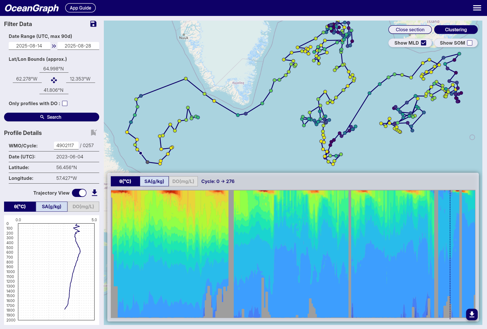
How to Read the Axes, Colors, and Float Path
The easiest way to read a time-series vertical section is to break it into four parts.
1. Read time across the section
The horizontal axis usually represents the sequence of observations through time.
That means neighboring columns or slices are not random. They are adjacent observations from the same float history or data sequence.
The first thing to ask is not “what is the absolute color here?” but “how does this pattern change from one cycle to the next?”
2. Read pressure or depth downward
The vertical axis shows the water column.
As with profile plots, higher pressure or greater depth means deeper water. Surface variability often appears near the top of the section, while deep stable structure appears lower down.
This makes it easier to separate shallow seasonal change from deeper persistence.
3. Treat color as the variable field, not as decoration
The color shading is the actual data pattern.
Depending on the selected parameter, color can reveal:
- A warm or cool surface layer
- A salinity maximum or minimum
- An oxygen-rich or oxygen-poor layer
- A boundary that shifts upward or downward over time
Read the colored regions as structure. Ask where strong gradients occur and whether they remain in similar depth ranges or move with time.
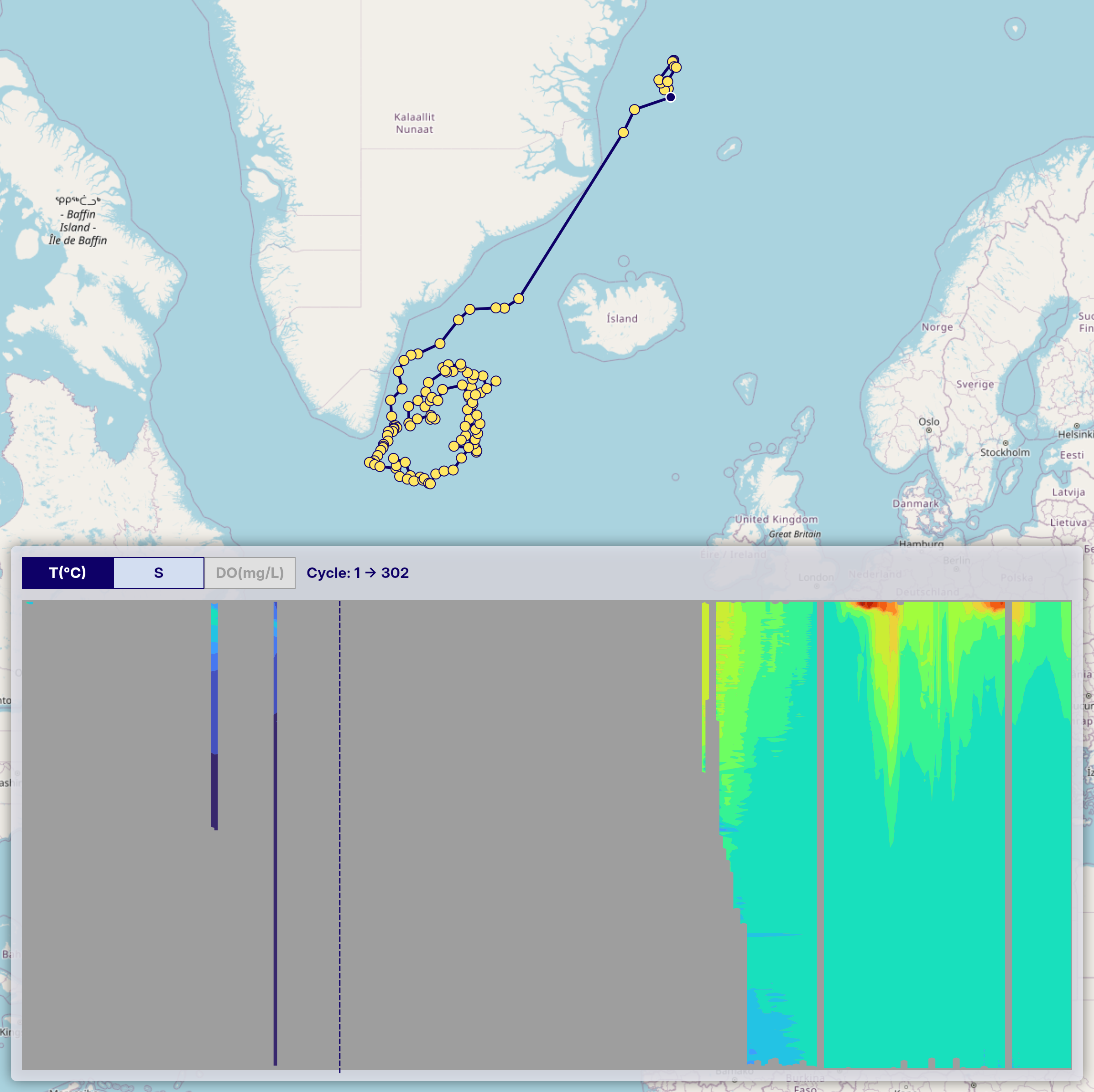
4. Keep the trajectory in mind
A time-series section is easier to interpret when you also know where the float moved.
If the platform drifts into a different water-mass region, the section can change for geographic reasons, not only seasonal ones. That is why trajectory context is important.
OceanGraph keeps this logic explicit in:
What a Section Reveals Better Than a Single Profile
A single profile is clear, but a section is better for pattern recognition across time.
A section helps you see:
- Whether the upper ocean changes while deep water stays similar
- Whether a gradient strengthens, weakens, shoals, or deepens
- Whether a feature appears across many cycles or only once
- Whether one odd profile is really unusual or part of a trend
Imagine a float in a subtropical region observed across several months. A section might show:
- A warm near-surface layer that thickens in one part of the record
- A strong thermocline that moves vertically over time
- Much smaller change below several hundred decibars
- A few cycles with sparse or missing values after QC
That is much harder to understand by opening the same profiles one at a time.
Sections also work well with diagnostic comparisons. If one part of the section looks unusual, the next step is often to open the matching profile and then check a T-S Diagrams in Oceanography Explained (With Examples) style view for property-space interpretation.
Missing or Gray Areas Do Not Always Mean “Nothing Happened”
One of the most common beginner mistakes is to treat blank or gray areas as if the ocean had no structure there.
That is not necessarily true.
In OceanGraph, time-series vertical sections are produced by interpolating irregularly spaced profile data onto a regular grid. Because of that, missing or masked areas can appear for several reasons:
- Original observations were not available in that part of the grid
- Quality control removed too many values
- The profiles were too sparse for interpolation to fill the section continuously
- BGC parameters had fewer valid observations than physical variables
So a gap may mean “not enough trustworthy data to color this area,” not “the water was empty” or “the variable was zero.”
OceanGraph’s limitation notes explain this in more detail:
For BGC-related variables, gaps can be even more common because fewer floats carry those sensors in the first place.
Common Beginner Mistakes
A few interpretation mistakes come up repeatedly.
Treating the section like a map
A section is not a horizontal map. It is a depth-through-time view tied to one float path or one observation sequence.
Over-interpreting interpolated patterns
Color gradients can look smooth even when the underlying observations are sparse. Use them as a guide, not as a reason to ignore data density and QC.
Ignoring the linked profile view
If one part of the section looks unusual, open the corresponding profile. Sections are strongest when used together with direct profile inspection.
Forgetting that variable coverage differs
Temperature and salinity are more widely available than many BGC variables. A section with many gaps may reflect sensor coverage and QC, not just poor plotting.
The Traditional Workflow: Assemble Many Profiles, Interpolate, Then Plot
If you build a time-series vertical section manually, the workflow usually looks like this:
- Gather many cycles from one float or sequence
- Read each profile from NetCDF
- Apply quality control decisions
- Interpolate the irregular observations onto a common grid
- Plot the gridded field
- Cross-check the section against the original profiles
That workflow is valid for research, but it is a heavy way to answer a first-pass question such as “does this float show stable deep structure and variable surface conditions?”
The harder part is not the plotting code itself. It is the need to manage interpolation, masking, and profile context before you have even decided whether the section is scientifically useful.
A Better First Step: Read the Section Interactively
If your immediate goal is interpretation, OceanGraph is often the better starting point.
A practical workflow is:
- Search for a float or relevant profile set.
- Select the float in the results or map view.
- Turn on trajectory mode.
- Open the vertical section view.
- Use the dashed line and profile linkage to inspect specific cycles more closely.
Useful related pages are:
That lets you move from “I think this float changes over time” to an actual section-based interpretation without building the plot manually.
Explore Time-Series Sections in OceanGraph
If you want to stop comparing isolated profiles and start reading change across time, OceanGraph is the direct next step.
Try with real Argo data -> OceanGraph
Explore profiles interactively
OceanGraph makes it easier to connect float trajectory, profile context, and section-based interpretation in one workflow.
Frequently Asked Questions
What does a time-series vertical section show?
It shows how one variable changes with depth across a sequence of observations over time. In Argo workflows, that usually means repeated profiles from one float.
Is a time-series vertical section the same as a ship transect?
Not exactly. The logic is similar because both show structure through a section-like view, but an Argo time-series section is built from repeated profiles collected over time as the float moves.
Why are there blank or gray areas in the section?
Usually because the original observations were sparse, quality control removed values, or interpolation could not fill the grid reliably. It does not automatically mean the ocean had no structure there.
When should I use a section instead of individual profiles?
Use a section when your question is about change across many cycles. Use individual profiles when you need to inspect one water column in detail.
Do I need Python to make sense of a section?
No. Python is useful for custom processing, but it does not have to be your first step if your goal is to understand the pattern first.
Conclusion
Time-series vertical sections are useful because they turn repeated profiles into a readable picture of change across time and depth. They are especially valuable in Argo workflows, where the key question is often not just what one profile looks like, but how the water column evolves from cycle to cycle.
For many learners, the fastest route is to inspect those sections interactively before building a manual gridding workflow. That is where OceanGraph is especially helpful.